6. Error Control Coding

6.1. Exercise 1 Hamming Distance

Consider the following error control code

Message	Codeword
\(s_1\)	\(c_1 = 00000\)
\(s_2\)	\(c_2 = 10011\)
\(s_3\)	\(c_3 = 11100\)
\(s_4\)	\(c_4 = 00111\)

Requirements:

• a). compute the minimum Hamming distance and indicate how many errors it can detect and how many errors it can correct, with the nearest neighbor decoding algorithm;

• b). considering two received codewords, \(\mathbf{r_1} = 11100\) and \(\mathbf{r_2} = 01111\), perform decoding and say if there are errors, and if so then correct the errors (find the correct codeword and indicate where the errors are located);

• c). Give an example of errors the code cannot detect, and another example of errors it can detect but it cannot correct, using the nearest neighbor decoding algorithm.

6.1.1. Solution

a). compute the minimum Hamming distance and indicate how many errors it can detect and how many errors it can correct, with the nearest neighbor decoding algorithm

The Hamming distance between two codewords is the number of bit differences between them. For example, the Hamming distance between \(000\) and \(110\) is \(d_H = 2\), because the first two bits are different.

The minimum Hamming distance of a code, \(d_{H_{min}}\), is is the smallest Hamming distance between any pair of codewords. It determines the number of errors the code can detect and correct using the nearest neighbor approach.

Therefore, we first have to compute the Hamming distance between all pairs of codewords, and find the minimum value.

\[\begin{split} \begin{align*} d_H(c_1, c_2) &= 3 (\textrm{ the first and last two bits are different}) \\ d_H(c_1, c_3) &= 3 \\ d_H(c_1, c_4) &= 3 \\ d_H(c_2, c_3) &= 4 \\ d_H(c_2, c_4) &= 2 \\ d_H(c_3, c_4) &= 4 \end{align*} \end{split}\]

The minimum Hamming distance is \(d_{H_{min}} = 2\), between \(c_2\) and \(c_4\).

The number of errors the code can detect is:

\[e_d = d_{H_{min}} - 1\]

so this code can detect \(2 - 1 = 1\) errors.

The number of errors the code can correct is:

\[e_c = \lfloor \frac{d_{H_{min}} - 1}{2} \rfloor\]

so this code can correct \(\lfloor \frac{2 - 1}{2} \rfloor = 0\) errors.

b). considering two received codewords, \(\mathbf{r_1} = 11100\) and \(\mathbf{r_2} = 01111\), perform decoding and say if there are errors, and if so then correct the errors (find the correct codeword and indicate where the errors are located)

The nearest neighbor decoding algorithm works as follows:

1. To detect if there are errors, we check if the received codeword is one of the codewords or not;if it is not, then there exist errors;

2. To fix errors, we compute the Hamming distance between the received codeword and all codewords, and select the codeword with the minimum distance. We assume that this should be the correct codeword; the differences from the received codeword are the errors.

Here, we take each received codeword separately.

\(\mathbf{r_1} = 11100\) is actual \(c_3\), so there are no errors.

\(\mathbf{r_2} = 01111\) is not in the table of codewords, so there are errors. We compute the Hamming distance between \(\mathbf{r_2}\) and all codewords:

\[\begin{split} \begin{align*} d_H(r_2, c_1) &= 4 \\ d_H(r_2, c_2) &= 3 \\ d_H(r_2, c_3) &= 3 \\ d_H(r_2, c_4) &= 1 \end{align*} \end{split}\]

The minimum distance is \(d_H(r_2, c_4) = 1\), so the correct codeword is \(c_4 = 00111\), and the error is in the second bit, which was \(0\) in the codeword, but was received as \(1\).

c). Give an example of errors the code cannot detect, and another example of errors it can detect but it cannot correct, using the nearest neighbor decoding algorithm

The code fails to detect errors if and only if the errors transform one codeword into another codeword. For example, when we send \(c_2 = 10011\) and there are two errors in the first and third positions, we receiver \(\mathbf{r} = 00111\), which is actually \(c_4\), so the code believes it to be correct.

An example of errors the code can detect but cannot correct properly is when the code detects the errors, but the nearest codeword is not the correct one, or there are two codewords equally close to the received codeword. For example, suppose we send \(c_2 = 10011\) and there is an error in the first position, so we receive \(\mathbf{r} = 00011\). This is not in the codeword table, so the code can detect that errors exist. When computing the nearest codeword, we have two codewords equally close to the received codeword:

\[\begin{split} \begin{align*} d_H(r, c_1) &= 2 \\ d_H(r, c_2) &= 1 \\ d_H(r, c_3) &= 5 \\ d_H(r, c_4) &= 1 \end{align*} \end{split}\]

The code will choose either \(c_2\) or \(c_4\) as the nearest codeword, but it cannot know which one is the correct one, so sometimes it will choose the wrong one and fail.

6.2. Exercise 2 Hamming Distance

a). Design a block code consisting of 4 codewords, with minimum codeword length, which is able to detect 3 errors in a codeword.

b). Design a block code consisting of 4 codewords, with minimum codeword length, which is able to correct 2 errors in a codeword.

6.2.1. Solution

a). Design a block code consisting of 4 codewords, with minimum codeword length, which is able to detect 3 errors in a codeword

To detect 3 errors in a codeword, we need the minimum Hamming distance to be at least 4. Therefore we need to come up with 4 codewords, such that the Hamming distance between any pair of them is at least 4. There is no rule here, we just use our imagination, and if we can’t find a solution, we can try to increase the codeword length.

One example:

Message	Codeword
\(s_1\)	\(c_1 = 000000\)
\(s_2\)	\(c_2 = 111100\)
\(s_3\)	\(c_3 = 110011\)
\(s_4\)	\(c_4 = 001111\)

b). Design a block code consisting of 4 codewords, with minimum codeword length, which is able to correct 2 errors in a codeword

To correct 2 errors in a codeword, we need the minimum Hamming distance to be at least 5, since \(\lfloor \frac{5 - 1}{2} \rfloor = 2\).

Therefore we need to come up with 4 codewords, such that the Hamming distance between any pair of them is at least 5. One example:

Message	Codeword
\(s_1\)	\(c_1 = 00000000\)
\(s_2\)	\(c_2 = 11111100\)
\(s_3\)	\(c_3 = 00011111\)
\(s_4\)	\(c_4 = 11100011\)

6.3. Exercise 3 Linear Block Codes

Consider a systematic code with generator matrix

\[\begin{split}[G] = \begin{bmatrix} 1 & 0 & 0 & 0 & 1 & 1 & 0 \\ 0 & 1 & 0 & 0 & 1 & 1 & 1 \\ 0 & 0 & 1 & 0 & 1 & 0 & 1 \\ 0 & 0 & 0 & 1 & 0 & 1 & 1 \\ \end{bmatrix}\end{split}\]

• a). Compute the codeword for sending the information bits \(\mathbf{i_2} = [1 0 1 1]\)

• b). Compute the control matrix \([H]\);

• c). We receive a sequence \(\mathbf{r} = 1010111\), which was encoded with this code. Find if there are errors in the received data, and, if yes, perform correction and retrieve the transmitted information bits.

• d). Find out how many errors this code can detect, and how many it can correct.

6.3.1. Solution

a). Compute the codeword for sending the information bits \(\mathbf{i_2} = [1 0 1 1]\)

When using a generator matrix \([G]\), we compute the codeword by multiplying the information word with the generator matrix:

Fig. 6.1 Computing the codeword by multiplying with \([G]\)

Note how the first part of \(G\) is the identity matrix, and this makes the first 4 bits of the codeword the same as the information word.

b). Compute the control matrix \([H]\)

When the generator matrix is in the form:

\[[G] = \begin{bmatrix} I_k & Q \end{bmatrix}\]

then the control matrix is given by:

\[[H] = \begin{bmatrix} Q^T & I_{n-k} \end{bmatrix}\]

where \(I_k\) is the identity matrix of size \(k\), \(Q\) is the other part of the generator matrix, \(Q^T\) is Q transposed, and \(I_{n-k}\) is the identity matrix of size \(n-k\).

In our case, we have:

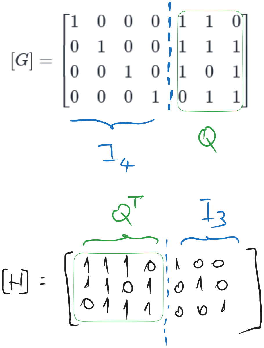
Fig. 6.2 Computing the control matrix \([H]\) from the generator matrix \([G]\) of a systematic code

c). We receive a sequence \(\mathbf{r} = 1010111\), which was encoded with this code. Find if there are errors in the received data, and, if yes, perform correction and retrieve the transmitted information bits

We first compute the syndrome \(\mathbf{z} = [H] \cdot \mathbf{r}^T\):

\[\begin{split} \mathbf{z} = \begin{bmatrix} 1 & 1 & 1 & 0 & 1 & 0 & 0 \\ 1 & 1 & 0 & 1 & 0 & 1 & 0 \\ 0 & 1 & 1 & 1 & 0 & 0 & 1 \\ \end{bmatrix} \cdot \begin{bmatrix} 1 \\ 0 \\ 1 \\ 0 \\ 1 \\ 1 \\ 1 \\ \end{bmatrix} = \begin{bmatrix} 1 \\ 0 \\ 0 \\ \end{bmatrix} \end{split}\]

If \(\mathbf{z} = 0\), then there are no errors. Here, \(\mathbf{z} \neq 0\), so there are errors detected.

To correct the errors, we need to find the error pattern \(\mathbf{e}\) such that \(\mathbf{z} = [H] \cdot \mathbf{e}^T\). For example, if there would be an error in the first bit, then we have:

\[\begin{split} \begin{bmatrix} 1 & 1 & 1 & 0 & 1 & 0 & 0 \\ 1 & 1 & 0 & 1 & 0 & 1 & 0 \\ 0 & 1 & 1 & 1 & 0 & 0 & 1 \\ \end{bmatrix} \cdot \begin{bmatrix} 1 \\ 0 \\ 0 \\ 0 \\ 0 \\ 0 \\ 0 \\ \end{bmatrix} = \begin{bmatrix} 1 \\ 1 \\ 0 \\ \end{bmatrix} \end{split}\]

This is not equal to our \(\mathbf{z}\), so the error is not in the first bit. We go on and try an error in the second bit, and so on. We can store the results in a look-up table, until we find the error pattern that matches the syndrome \(\mathbf{z}\):

Error pattern	Syndrome
\([1 0 0 0 0 0 0]\)	\([1 1 0]\)
\([0 1 0 0 0 0 0]\)	\([1 1 1]\)
\([0 0 1 0 0 0 0]\)	\([1 0 1]\)
\([0 0 0 1 0 0 0]\)	\([0 1 1]\)
\([0 0 0 0 1 0 0]\)	\([1 0 0]\)

It is easy to see that for one error bit on the \(k\)-th position the result is the \(k\)-th column \([H]\). Thus, since our syndrome \(\mathbf{z} = [1 0 0]^T\) is the 5th column of \([H]\), the error is in the 5th position, so we have \(\mathbf{e} = [0 0 0 0 1 0 0]\).

Therefore the error is on the 5th position, we change that bit and find the correct codeword:

\[ \mathbf{c} = \mathbf{r} \oplus \mathbf{e} = [1 0 1 0 0 1 1] \]

Remembering from a). that the first 4 bits of the codeword are the information bits, we find the transmitted information bits are:

\[\mathbf{i} = [1 0 1 0]\]

d). Find out how many errors this code can detect, and how many it can correct

This is from the theory of linear block codes.

A code can detect up to \(e_d\) errors if and only if the sum of any \(e_d\) or fewer columns from \([H]\) is not equal to the zero vector. Here, we have:

• all columns of \([H]\) are non-zero, so we can detect at least 1 error;

• the sum of any 2 columns is non-zero, because all columns are different from each other, so we can detect at least 2 errors;

• there exist 3 columns for which the sum is zero (for example the first plus fifth plus sixth columns), so the code cannot detect 3 errors.

So, our code can detect up to \(e_d = 2\) errors.

A code can correct up to \(e_c\) errors if and only if the sum of any \(e_c\) or fewer columns is always unique (not equal to the sum of any other \(e_c\) or fewer columns).

Here, we have:

• every column is unique, so we can correct at least 1 error;

• the sum of 2 columns is not unique: for example, the first column is equal to the sum of the fifth and sixth columns, so we cannot correct 2 errors.

So, our code can correct up to \(e_c = 1\) error.

6.4. Exercise 4 Hamming Codes - encoding

Compute the codewords for transmitting the information words \(\mathbf{i_1} = [1 0 0 1]\) with the Hamming (7,4) code, and \(\mathbf{i_2} = [1 1 1 0]\) with the Hamming (8,4) SECDED code.

6.4.1. Solution

Hamming codes are linear block codes, but we won’t use the generator matrix because it is hard to remember. Instead, for the Hamming code, we need to know (from the theory) the control matrix \([H]\) and the structure of the codeword.

a). Hamming (7,4) code

The \([H]\) matrix of a Hamming code contains all the numbers from 1 to \(n\) in binary, written as columns, from \([0 ... 0 1]\) to \([1 1 ... 1]\).

For the Hamming (7,4) code, we have all the numbers from 1 to 7 in binary, written on 3 bits, as columns:

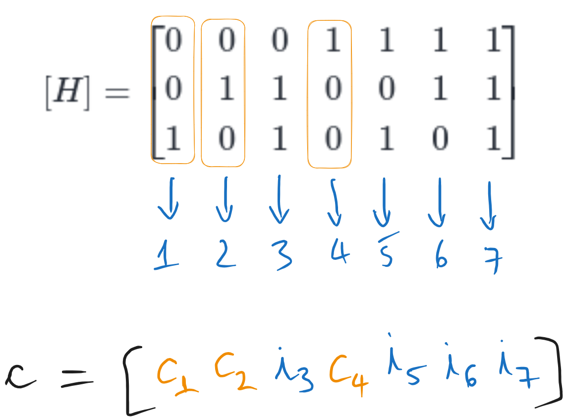
Fig. 6.3 The control matrix \([H]\) of the Hamming (7,4) code and the structure of the codeword

The codeword has the same length as \([H]\), and the bits corresponding to the columns with a single \(1\) in the column are the control bits, and the others are information bits. Thus, for the Hamming (7,4) code, bits 1, 2, and 4 are control bits, and bits 3, 5, 6, and 7 are information bits.

We can write the codeword as:

\[\mathbf{c} = [c_1 c_2 i_3 c_4 i_5 i_6 i_7]\]

where \(i\) or \(c\) means information or control bit, and the index is the position in the codeword.

To find the codeword, we replace the information bits in the codeword with the actual values, and we put the condition that the syndrome \(\mathbf{z} = [H] \cdot \mathbf{c}^T\) is zero, since this is the condition for a valid codeword.

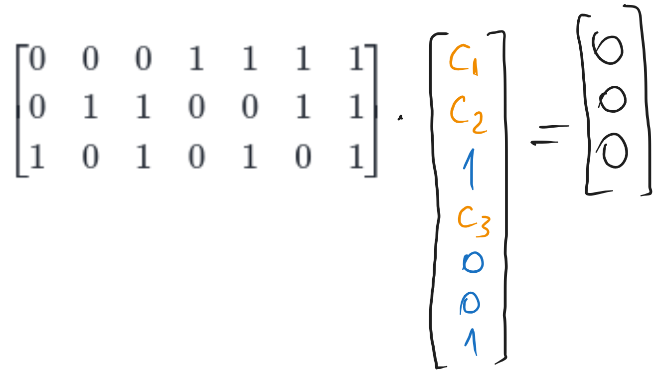
Fig. 6.4 Computing the codeword for the Hamming (7,4) code

Writing the equations, we have:

\[\begin{split} \begin{align*} c_3 \oplus 0 \oplus 0 \oplus 1 &= 0 => c_3 = 1 \\ c_2 \oplus 1 \oplus 0 \oplus 1 &= 0 => c_2 = 0 \\ c_1 \oplus 1 \oplus 0 \oplus 1 &= 0 => c_1 = 0 \\ \end{align*} \end{split}\]

So the codeword is:

\[\mathbf{c} = [0 0 1 1 0 0 1]\]

b). Hamming (8,4) SECDED code

The SECDED code is an extension of the Hamming code, which adds an extra control bit \(c_0\) in front, which is the parity bit of the whole codeword.

Therefore, we can compute the codeword for the Hamming (7,4) and then add the parity bit in front.

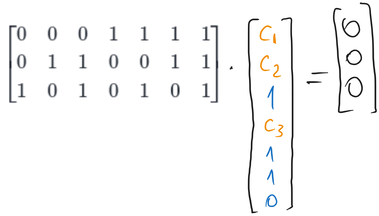
Fig. 6.5 Computing another codeword for the Hamming (7,4) code

\[\begin{split} \begin{align*} c_3 \oplus 1 \oplus 1 \oplus 0 &= 0 => c_3 = 0 \\ c_2 \oplus 1 \oplus 1 \oplus 0 &= 0 => c_2 = 0 \\ c_1 \oplus 1 \oplus 1 \oplus 0 &= 0 => c_1 = 0 \\ \end{align*} \end{split}\]

So the Hamming (7,4) codeword is \(\mathbf{c} = [0 0 1 0 1 1 0]\)

For the Hamming (8,4) SECDED code, we compute the parity bit of the above sequence, which is \(1\) in this case, and we add it in front as a new control bit \(c_0\):

\[\mathbf{c} = [1 0 0 1 0 1 1 0]\]

6.5. Exercise 5 Hamming Codes - decoding

We receive a sequence \(\mathbf{r} = 1010111\), which was encoded with the Hamming (7,4) code. Find if there are errors in the received data, and, if yes, perform correction and retrieve the transmitted information bits.

6.5.1. Solution

We need to know the control matrix \([H]\) of the Hamming (7,4) code, and the structure of the codeword, as in the previous exercise.

To check if there are errors, we compute the syndrome \(\mathbf{z} = [H] \cdot \mathbf{r}^T\), and we check if \(\mathbf{z} = 0\) or not.

\[\begin{split} \mathbf{z} = \begin{bmatrix} 0 & 0 & 0 & 1 & 1 & 1 & 1 \\ 0 & 1 & 1 & 0 & 0 & 1 & 1 \\ 1 & 0 & 1 & 0 & 1 & 0 & 1 \\ \end{bmatrix} \cdot \begin{bmatrix} 1 \\ 0 \\ 1 \\ 0 \\ 1 \\ 1 \\ 1 \\ \end{bmatrix} = \begin{bmatrix} 1 \\ 1 \\ 0 \\ \end{bmatrix} \end{split}\]

Since \(\mathbf{z} \neq 0\), there are errors in the received data.

To fix the errors, the syndrome gives the position of the error bit, in binary. Here, we have \(\mathbf{z} = [1 1 0]^T\), which is the binary representation of the number \(6\). The error in on the 6th position, so we have \(\mathbf{e} = [0 0 0 0 0 1 0]\).

The correct codeword is found by toggling back the 6th bit of the received codeword:

\[\mathbf{c} = \mathbf{r} \oplus \mathbf{e} = [1 0 1 0 1 0 1]\]

For Hamming(7,4) the information bits are the bits in the positions 3, 5, 6, and 7, so we have:

\[\mathbf{i} = [1 1 0 1]\]

6.6. Exercise 6 Hamming SECDED Codes - decoding

We receive a sequence \(\mathbf{r} = 10101011\), which was encoded with the Hamming (8,4) SECDED code. Find if there are errors in the received data, and, if yes, perform correction and retrieve the transmitted information bits.

6.6.1. Solution

We need to know the control matrix \([H]\) of the Hamming (8,4) SECDED code, and the structure of the codeword.

The control matrix \([\tilde{H}]\) of the SECDED code is the \([H]\) for the normal Hamming code, but with an extra row of \(1\)s at the top, and an extra column of \(0\)s in front.

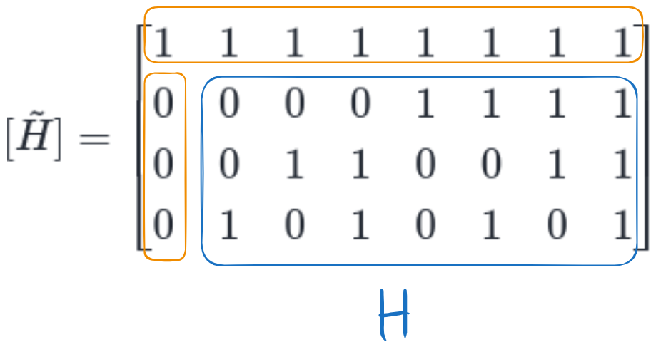
Fig. 6.6 The control matrix \([\tilde{H}]\) of the Hamming (8,4) SECDED code

The codeword is the normal Hamming codeword, but with an extra control bit \(c_0\) in front:

\[\mathbf{c} = [c_0 c_1 c_2 i_3 c_4 i_5 i_6 i_7]\]

We compute the syndrome in the same way as before, but note that it has one more bit now:

\[\begin{split} \mathbf{z} = [\tilde{H}] \cdot \mathbf{r}^T = \begin{bmatrix} 1 & 1 & 1 & 1 & 1 & 1 & 1 & 1 \\ 0 & 0 & 0 & 0 & 1 & 1 & 1 & 1 \\ 0 & 0 & 1 & 1 & 0 & 0 & 1 & 1 \\ 0 & 1 & 0 & 1 & 0 & 1 & 0 & 1\\ \end{bmatrix} \cdot \begin{bmatrix} 1 \\ 0 \\ 1 \\ 0 \\ 1 \\ 0 \\ 1 \\ 1 \\ \end{bmatrix} = \begin{bmatrix} 1 \\ 1 \\ 1 \\ 1 \\ \end{bmatrix} \end{split}\]

The decoding algorithm is:

1. If \(\mathbf{z} = 0\), then there are no errors;

2. If \(\mathbf{z} \neq 0\), then there are errors

   1. If the first bit of \(\mathbf{z}\) is \(1\), then there is a single error, and its position is given by the other three bits in \(\mathbf{z}\), just like in normal Hamming codes; (position goes from 0 to 7 now, 0 = first bit, 7 = last bit).

   2. If the first bit of \(\mathbf{z}\) is \(0\), then there are two errors, and we cannot correct them, so we don’t do anything.

Here, the first bit of \(\mathbf{z}\) is \(1\), so there is a single error, on position \(111 = 7\), which means the last bit. The correct codeword is:

\[\mathbf{c} = \mathbf{r} \oplus \mathbf{e} = [1 0 1 0 1 0 1 1] \oplus [0 0 0 0 0 0 0 1] = [1 0 1 0 1 0 1 0]\]

The four information bits are \(i_3, i_5, i_6, i_7\), so we have:

\[\mathbf{i} = [0 0 1 0]\]

(remember that the first bit is \(c_0\) now, so \(i_3\) is the fourth bit etc.).

6.7. Exercise 7 Hamming Codes - errors

Give an example of errors which the Hamming (15, 11) is not able to detect. Give another example of errors which the Hamming (15, 11) is able to detect, but is not able to fix them correctly.

6.7.1. Solution

The control matrix \([H]\) of the Hamming (15, 11) code contains numbers from 1 to \(n\) written on 4 bits, so they go from 1 to 15:

\[\begin{split}[H] = \begin{bmatrix} 0 & 0 & 0 & 0 & 0 & 0 & 0 & 1 & 1 & 1 & 1 & 1 & 1 & 1 & 1 \\ 0 & 0 & 0 & 1 & 1 & 1 & 1 & 0 & 0 & 0 & 0 & 1 & 1 & 1 & 1 \\ 0 & 1 & 1 & 0 & 0 & 1 & 1 & 0 & 0 & 1 & 1 & 0 & 0 & 1 & 1 \\ 1 & 0 & 1 & 0 & 1 & 0 & 1 & 0 & 1 & 0 & 1 & 0 & 1 & 0 & 1 \\ \end{bmatrix} \end{split}\]

Hamming codes are linear block codes, so the same rules apply as for linear block codes. An error pattern goes undetected if the sum of the corresponding columns of \([H]\) is equal to the zero vector. For example, if we have three errors, on the first three bits, then the error pattern is:

\[\mathbf{e} = [1 1 1 0 0 0 0 0 0 0 0 0 0 0 0]\]

The syndrome is:

\[\begin{split} \mathbf{z} = [H] \cdot \mathbf{e}^T = \begin{bmatrix} 0 & 0 & 0 & 0 & 0 & 0 & 0 & 1 & 1 & 1 & 1 & 1 & 1 & 1 & 1 \\ 0 & 0 & 0 & 1 & 1 & 1 & 1 & 0 & 0 & 0 & 0 & 1 & 1 & 1 & 1 \\ 0 & 1 & 1 & 0 & 0 & 1 & 1 & 0 & 0 & 1 & 1 & 0 & 0 & 1 & 1 \\ 1 & 0 & 1 & 0 & 1 & 0 & 1 & 0 & 1 & 0 & 1 & 0 & 1 & 0 & 1 \\ \end{bmatrix} \cdot \begin{bmatrix} 1 \\ 1 \\ 1 \\ 0 \\ 0 \\ 0 \\ 0 \\ 0 \\ 0 \\ 0 \\ 0 \\ 0 \\ 0 \\ 0 \\ 0 \\ \end{bmatrix} = \begin{bmatrix} 0 \\ 0 \\ 0 \\ \end{bmatrix} \end{split}\]

and the decoder believes that there are no errors.

The code is not able to fix errors correctly if the syndrome corresponds to a single error which is not the true one. For example, if we have two errors on the first and second bits, then the error pattern is: $\(\mathbf{e} = [1 1 0 0 0 0 0 0 0 0 0 0 0 0 0]\)$

\[\begin{split} \mathbf{z} = [H] \cdot \mathbf{e}^T = \begin{bmatrix} 0 & 0 & 0 & 0 & 0 & 0 & 0 & 1 & 1 & 1 & 1 & 1 & 1 & 1 & 1 \\ 0 & 0 & 0 & 1 & 1 & 1 & 1 & 0 & 0 & 0 & 0 & 1 & 1 & 1 & 1 \\ 0 & 1 & 1 & 0 & 0 & 1 & 1 & 0 & 0 & 1 & 1 & 0 & 0 & 1 & 1 \\ 1 & 0 & 1 & 0 & 1 & 0 & 1 & 0 & 1 & 0 & 1 & 0 & 1 & 0 & 1 \\ \end{bmatrix} \cdot \begin{bmatrix} 1 \\ 1 \\ 0 \\ 0 \\ 0 \\ 0 \\ 0 \\ 0 \\ 0 \\ 0 \\ 0 \\ 0 \\ 0 \\ 0 \\ 0 \\ \end{bmatrix} = \begin{bmatrix} 0 \\ 1 \\ 1 \\ \end{bmatrix} \end{split}\]

The syndrome \(\mathbf{z} = [0 1 1]^T\) corresponds to the error on the 3rd position, so the decoder will believe that the error is on the 3rd position, which is not true.

6.8. Exercise 8 Cyclic Codes - encoding

Find the non-systematic and then the systematic cyclic codeword for the sequence \(\mathbf{i} = [1 0 1 0 0 0 1 1 0 0]\) (first bit is LSB), considering a cyclic code with generator polynomial \(g(x) = 1\oplus x \oplus x^3\).

• a). Do it “the mathematical way” (with polynomials)

• b). Do it “the programming way” (XOR-ing bit sequences)

6.8.1. Solution

a). “the mathematical way” (with polynomials)

We first convert the binary sequence into a polynomial. The LSB corresponds to \(x^0\), and the MSB corresponds to the highest degree.

\[\begin{split} \mathbf{i} = [1 0 1 0 0 0 1 1 0 0] &\Rightarrow i(x) = 1 \oplus x^2 \oplus x^6 \oplus x^7 \\ \end{split}\]

Also, we note that the generator polynomial has degree \(3\), which means that the codeword is 3 bits longer than the information word. Since the information word given length \(k = 10\), the codeword will have \(n = k + 3 = 13\) bits.

Degree of generator polynomial

For cyclic codes, the degree of the generator polynomial \(g(x)\) is the increase in number of bits due to the code.

Non-systematic codeword

The non-systematic codeword is computed by multiplying \(i(x)\) with \(g(x)\):

\[\begin{split} \begin{align*} c(x) &= i(x) \cdot g(x) \\ &= (1 \oplus x^2 \oplus x^6 \oplus x^7) \cdot (1 \oplus x \oplus x^3) \\ &= 1 \oplus x \oplus x^3 \oplus x^2 \oplus x^3 \oplus x^5 \oplus x^6 \oplus x^7 \oplus x^9 \oplus x^7 \oplus x^8 \oplus x^{10} \\ &= 1 \oplus x \oplus x^2 \oplus x^5 \oplus x^6 \oplus x^8 \oplus x^9 \oplus x^{10} \\ \end{align*} \end{split}\]

Note that equal terms cancel out (i.e. \(x^3 \oplus x^3 = 0\)).

We now convert back the polynomial into a binary sequence, by listing the coefficients. However, we only have 11 coefficients (from \(x^0\) to \(x^{10}\)), but we know we need a codeword of length \(n = 13\), so we add two zeros at the end, to make it of length \(n = 13\). These correspond to missing terms \(0 x^{11} + 0 x^{12}\), which could have appeared in the polynomial, but happened to be zero.

\[ \mathbf{c} = [1 1 1 0 0 1 1 0 1 1 1 0 0] \]

Systematic codeword

The systematic codeword is computed as:

\[ c(x) = x^{n-k} \cdot i(x) + b(x) \]

where \(n-k\) is the degree of \(g(x)\) (\(n-k = 3\) in our case), and \(b(x)\) is the remainder of the division of \(x^{n-k} \cdot i(x)\) by \(g(x)\).

In our case, we have:

\[ x^{n-k} \cdot i(x) = x^3 \cdot (1 \oplus x^2 \oplus x^6 \oplus x^7) = x^3 \oplus x^5 \oplus x^9 \oplus x^{10} \]

We divide this to \(g(x)\) to find the remainder. Note that the polynomial division requires writing the polynomials in descending order.

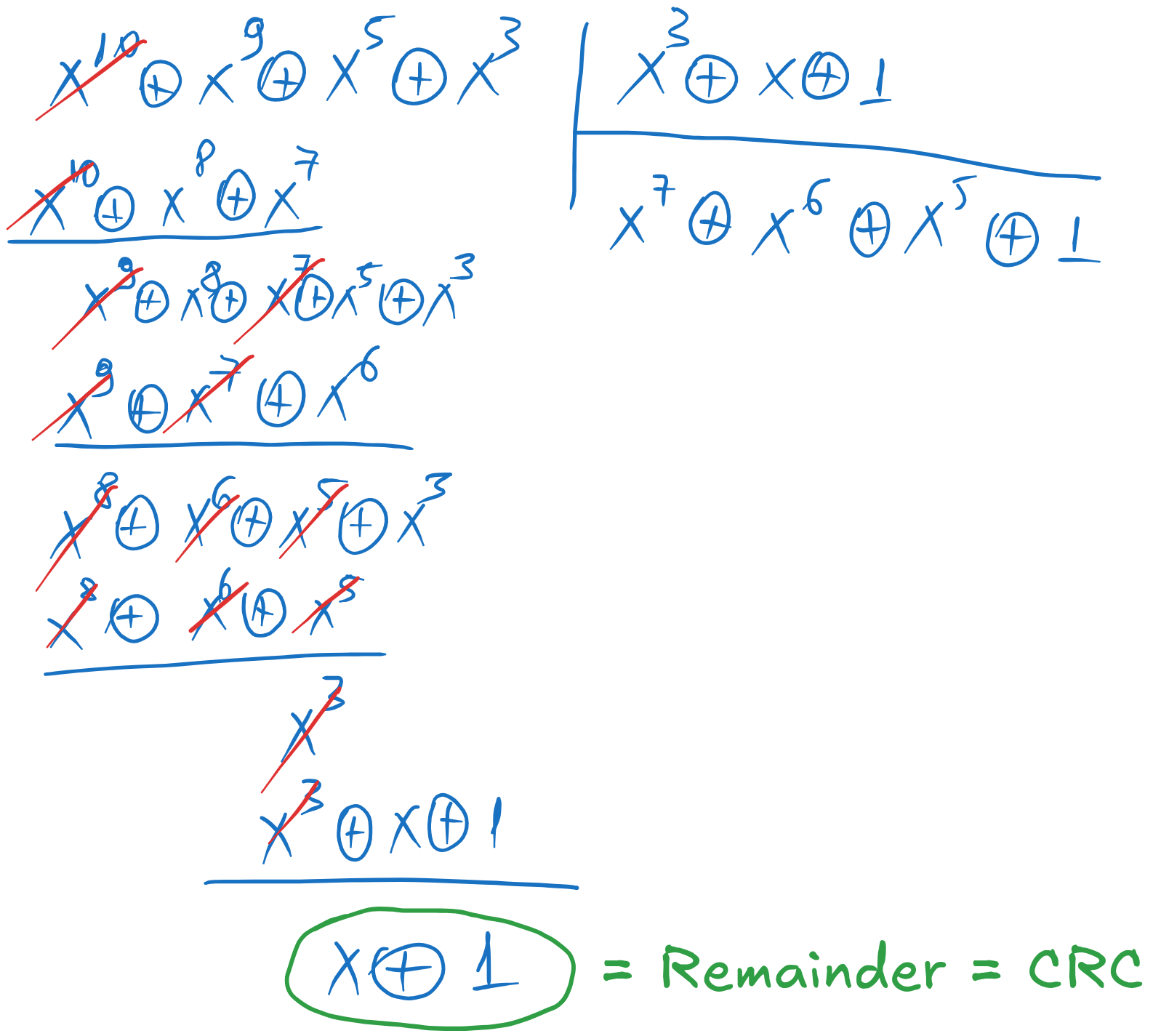
Fig. 6.7 Computing the remainder of the division of \(x^{n-k} \cdot i(x)\) by \(g(x)\)

The remainder is \(1 \oplus x\). We add the remainder to \(x^{n-k} \cdot i(x)\) to find the systematic codeword polynomial:

\[ c(x) = 1 \oplus x \oplus x^3 \oplus x^5 \oplus x^9 \oplus x^{10} \]

We read out the coefficients of the polynomial to get the codeword in binary, appending two zeros at the end to obtain the prescribed length \(n = 13\):

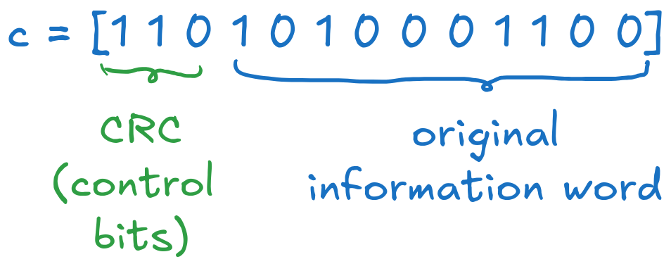
Fig. 6.8 Final systematic codeword

b). “the programming way” (XOR-ing bit sequences)

We use this only for the systematic codeword. This method is equivalent to the mathematical way, but it is easier to implement as an algorithm on binary sequences.

We start from the information word and the generator polynomial written in binary, from MSB to LSB, so in our case in reverse order.

\[\begin{split} \begin{align*} \mathbf{i} &= [0 0 1 1 0 0 0 1 0 1] \\ \mathbf{g} &= [1 0 1 1] \\ \end{align*} \end{split}\]

We extend the information word with \(n-k = 3\) zeros at the end, initialized with 0, to make it of length \(n = 13\), as illustrated in the image below.

The procedure is as follows:

1. Locate the first \(1\) in \(\mathbf{i}\)

2. Under it write the generator sequence \(\mathbf{g}\)

3. Add the two sequences using XOR. Note that the first \(1\) is cancelled out.

4. Locate the next \(1\) in the resulting sequence, and repeat.

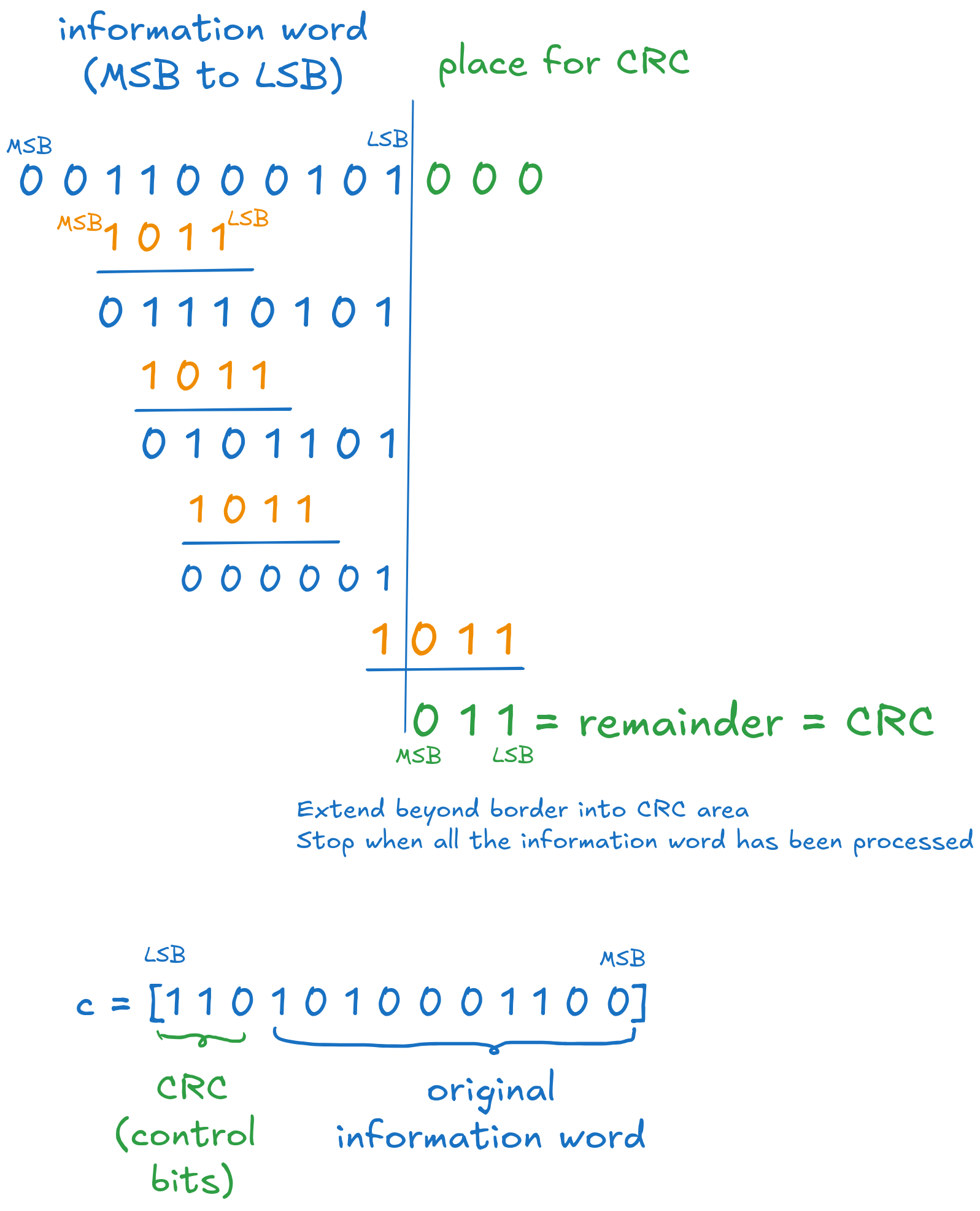
Fig. 6.9 Final systematic codeword

We stop when we reached the end of the information word. The three bits obtained at the end are control bits (i.e. the CRC, the remainder of the division).

Append the control bits at the LSB side of the information word to get the systematic codeword.

We revert the sequence afterwards, to get the final codeword in the original order (here, from LSB to MSB).

Explanation

This binary procedure is nothing else than the polynomial division we did earlier, but, instead of writing the powers \(x^k\) explicitly, we rely on the position of the bits to give us the power implicitly.

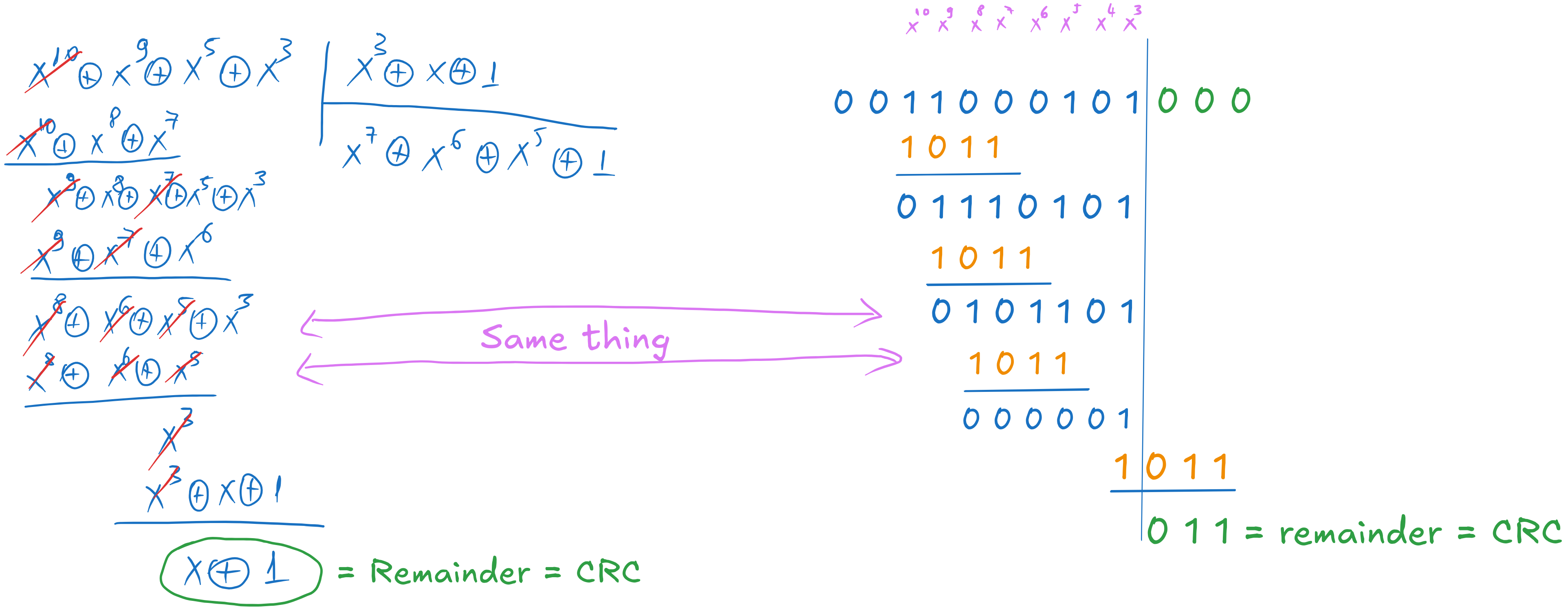
Fig. 6.10 Equivalence between polynomial division and binary algorithm

6.9. Exercise 9 Cyclic Codes - decoding

We receive a sequence \(\mathbf{r} = 101011100101\) (first bit is the LSB), which was encoded with a systematic cyclic code with generator polynomial \(g(x) = 1 \oplus x^2 \oplus x^3\). Find if there are errors in the received data, and, if yes, perform correction and retrieve the transmitted information bits.

• a). Do it “the mathematical way” (with polynomials)

• b). Do it “the programming way” (XOR-ing bit sequences)

6.9.1. Solution

a). “the mathematical way” (with polynomials)

We convert the received sequence into a polynomial, as before:

\[ \mathbf{r} = [1 0 1 0 1 1 1 0 0 1 0 1] \Rightarrow r(x) = 1 \oplus x^2 \oplus x^4 \oplus x^5 \oplus x^6 \oplus x^9 \oplus x^{11} \]

To check for errors, we divide \(r(x)\) by \(g(x)\), and we check the remainder. If it is zero, then there are no errors. If not, then there are errors. Remember to arrange the polynomials in descending order of powers (MSB to LSB)

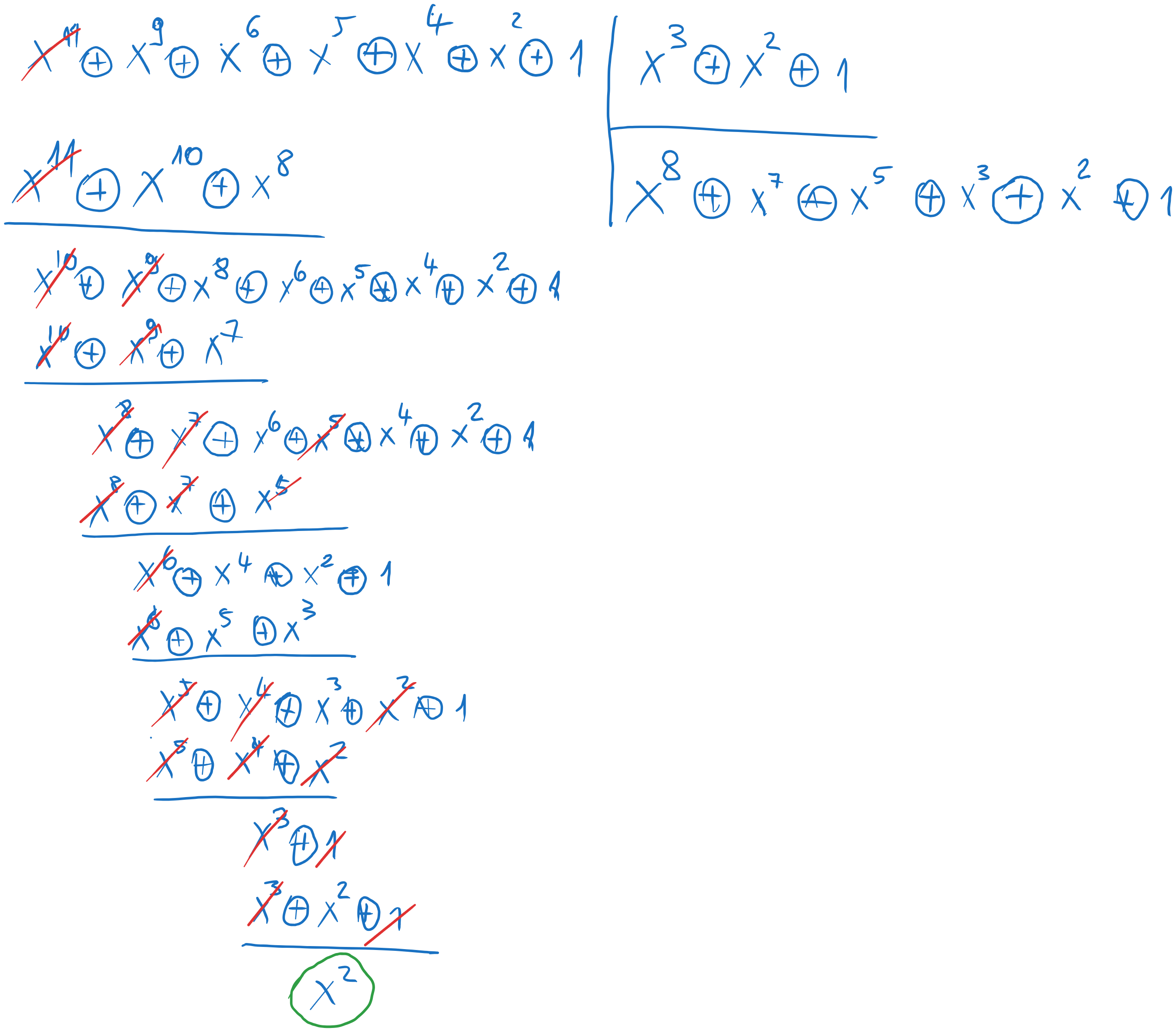
Fig. 6.11 Polynomial division at decoding

In our case we have the remainder \(b(x) = x^2\), so there are errors.

To correct the errors, we need to find the error pattern \(\mathbf{e}\) which produces the same remainder when divided by \(g(x)\).

As for linear block codes, we try all possible error patterns with 1 error, then with 2 errors, and so on, until we find the one that produces the same remainder.

The error patterns with 1 error are \(1\), \(x\), \(x^2\), \(x^3\) … \(x^{11}\), so we take each one and we divide it by \(g(x)\) to find the remainder, until the remainder is equal to \(b(x) = x^2\).

Error pattern	Remainder
\([1 0 0 0 0 0 0 0 0 0 0 0] = 1\)	\([1 0 0] = 1\)
\([0 1 0 0 0 0 0 0 0 0 0 0] = x\)	\([0 1 0] = x\)
\([0 0 1 0 0 0 0 0 0 0 0 0] = x^2\)	\([0 0 1] = x^2\)

The third error pattern matches, so we have \(\mathbf{e} = [0 0 1 0 0 0 0 0 0 0 0 0]\), the error being on the third bit.

The correct codeword is:

\[ \mathbf{c} = \mathbf{r} \oplus \mathbf{e} = [1 0 1 0 1 1 1 0 0 1 0 1] \oplus [0 0 1 0 0 0 0 0 0 0 0 0] = [1 0 0 0 1 1 1 0 0 1 0 1] \]

We know that the first 3 bits on the LSB side are the CRC, so the other bits are the information bits:

\[ \mathbf{i} = [0 1 1 1 0 0 1 0 1] \]

b). “the programming way” (XOR-ing bit sequences)

We can use the binary algorithm instead of the division, in the same way as we did before.

6.10. Exercise 7 Cyclic Codes - general

We do cyclic coding on information words of length \(k = 8\) bits. We want the coding rate \(R\) to be at most \(0.6\). What degree must the generator polynomial \(g(x)\) have?

6.10.1. Solution

The coding rate \(R\) is:

\[ R = \frac{k}{n}\]

where \(k\) is the length of the information word, and \(n\) is the length of the codeword.

If \(k = 8\) and \(R \leq 0.6\), this implies a lower limit of \(n\):

\[ \frac{8}{n} \leq 0.6 \implies n \geq \frac{8}{0.6} \approx 13.33 \]

The degree of the generator polynomial \(g(x)\) is \(n - k\), so we have:

\[ \text{degree}(g(x)) = n - k \geq 13.33 - 8 = 5.33 \]

Since the degree must be an integer, we round it up to the next integer. Therefore, the degree of the generator polynomial must be at least \(6\).