4. Discrete Information Sources

4.1. Exercise 1 DMS entropy

Compute the entropy of the following distribution:

\[ \sV{S}{\frac{1}{2}}{0}{\frac{1}{8}}{\frac{1}{4}}{\frac{1}{8}} \]

4.1.1. Solution

The entropy of a DMS is given by:

\[ H(S) = - \sum_{i=1}^{n} p(s_i) \log_2 p(s_i) \]

In this case, we have:

\[\begin{split} \begin{aligned} H(S) & = - \frac{1}{2} \log_2 \frac{1}{2} + 0 \log_2 0 + \frac{1}{8} \log_2 \frac{1}{8} + \frac{1}{4} \log_2 \frac{1}{4} + \frac{1}{8} \log_2 \frac{1}{8} \\ & = - \frac{1}{2} (-1) - 0 - \frac{1}{8} (-3) - \frac{1}{4} (-2) - \frac{1}{8} (-3) \\ & = \frac{1}{2} + \frac{3}{8} + \frac{1}{2} + \frac{3}{8} \\ & = 1.75 \, \text{bits} \end{aligned} \end{split}\]

When probability is zero

Note the situation when a probability is 0, as we have here \(p(s_2) = 0\). This is a special case, because simply applying the formula would result in a term \(0 \log_2 0 = 0 \cdot \infty\), which is undefined.

The value of this term can be found as a limit, using l’Hôpital’s rule:

\[\begin{split} \begin{aligned} \lim_{p \to 0} p \log_2 p &= \lim_{p \to 0} \frac{\log_2 p}{\frac{1}{p}} \\ &= \lim_{p \to 0} \frac{\frac{1}{p \ln 2}}{-\frac{1}{p^2}} \\ &= \lim_{p \to 0} \frac{-p}{\ln 2} \\ &= 0 \end{aligned} \end{split}\]

Thus, a probability of zero does not contribute at all to the entropy, and can be safely ignored.

4.2. Exercise 2 Optimal questions

Consider the following game: I think of a number between 1 and 8 (each number has equal chances), and you have to guess it by asking yes/no questions.

Answer the following questions:

• a). How much uncertainty does the problem have?

• b). How is the best way to ask questions? Why?

• c). On average, what is the number of questions required to find the number?

• d). What if the questions are not asked in the best way?

4.2.1. Solution

a). How much uncertainty does the problem have?

The problem can be modeled as a DMS with 8 equiprobable messages:

\[ \sVIII{S}{\fIoVIII}{\fIoVIII}{\fIoVIII}{\fIoVIII}{\fIoVIII}{\fIoVIII}{\fIoVIII}{\fIoVIII} \]

The uncertainty of the problem is given by the entropy of this source:

\[ H(S) = - \sum_{i=1}^{8} \frac{1}{8} \log_2 \frac{1}{8} = 3 \, \text{bits} \]

b). How is the best way to ask questions? Why?

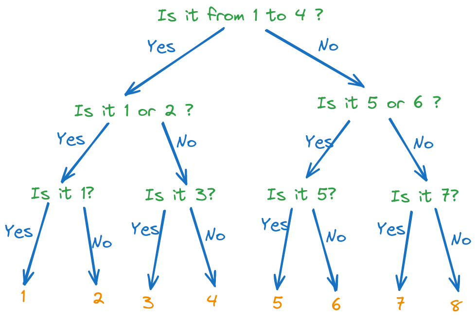
The best way to ask questions is to ask questions that split the set of possible numbers in two sets of equal probability. This is because every answer you obtain to a question behaves like a binary source, and this provides maximum information when the probabilities are equal:

\[ \snII{S}{Yes}{\frac{1}{2}}{No}{\frac{1}{2}} \]

Thus, the best way to ask questions is to maximize the entropy of the source at each step.

Fig. 4.1 Optimal decision tree for guessing a number between 1 and 8

c). On average, what is the number of questions required to find the number?

With the optimal questions, the number of questions required to find the number is always 3. This is because the entropy of the source is 3 bits, and the entropy of an answer is always 1 bit.

d). What if the questions are not asked in the best way?

This is just discussion during lecture.

If questions are not asked in the best way, the Yes/No answers will not have equal probabilities, and therefore the answers will provide, on average, less than 1 bit of information. Therefore the number of questions required to find the number will be more than three.

4.3. Exercise 3 Optimal decision tree

What is the optimal decision tree for guessing a number chosen according to the following distribution:

\[ \sIV{S}{\fIoII}{\fIoIV}{\fIoVIII}{\fIoVIII} \]

4.3.1. Solution

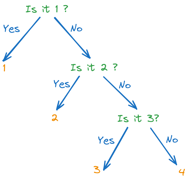
The difference with the previous case is that the probabilities are not equal. But we still use the same principle: we want to maximize the entropy at each step, which means that we want to split the set of possible numbers in two sets of equal probability. This corresponds to the following optimal decision tree:

Fig. 4.2 Optimal decision tree for guessing a number between 1 and 4

4.4. Exercise 4 Optimal decision tree

What is the optimal decision tree for guessing a number chosen according to the following distribution:

\[ \sIV{S}{0.14}{0.29}{0.4}{0.17} \]

4.4.1. Solution

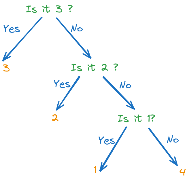
We still use the same principle as before. However, we cannot split the set of probabilities into equal amounts every time. Instead, we try to split them into sums which are as close to each other as possible, even though a perfect split is not always possible.

A good way to ask questions is shown below:

Fig. 4.3 Optimal decision tree for guessing a number between 1 and 4

4.5. Exercise 5 DMS

A DMS has the following distribution

\[ \sV{S}{\frac{1}{2}}{0}{\frac{1}{8}}{\frac{1}{4}}{\frac{1}{8}} \]

• a). Compute the information of message \(s_1\), \(s_2\) and \(s_3\)

• b). Compute the average information of a message of the source

• c). Compute the efficiency, absolute redundancy and relative redundancy of the source

• d). Compute the probability of generating the sequence \(s_1 s_4 s_3 s_1\)

4.5.1. Solution

a). Compute the information of message \(s_1\), \(s_2\) and \(s_3\)

The information of a message is given \(- \log_2 p(s_i)\), so we have:

\[\begin{split} \begin{aligned} i(s_1) & = - \log_2 \frac{1}{2} = 1 \, \text{bit} \\ i(s_2) & = - \log_2 0 = \infty \, \text{bits} \\ i(s_3) & = - \log_2 \frac{1}{8} = 3 \, \text{bits} \end{aligned} \end{split}\]

b). Compute the average information of a message of the source

The average information of a message is the entropy:

\[ H(S) = - \sum_{i=1}^{5} p(s_i) \log_2 p(s_i) = 1.75 \, \text{bits} \]

c). Compute the efficiency, absolute redundancy and relative redundancy of the source

For a DMS with 5 messages, the maximum entropy is \(\log_2 5 = 2.32 \, \text{bits}\).

Therefore we have:

\[\begin{split} \begin{aligned} \eta &= \frac{H(S)}{H_{max}} = \frac{1.75}{2.32} = ... \\ R &= H_{max} - H(S) = 2.32 - 1.75 = 0.57 \text{bits} \\ \rho &= \frac{H_{max} - H(S)}{H_{max}} = \frac{0.57}{2.32} = ... \end{aligned} \end{split}\]

d). Compute the probability of generating the sequence \(s_1 s_4 s_3 s_1\)

Since the source is memoryless, the messages are independent, and the probability of generating the sequence is the product of each message probability:

\[ P(s_1 s_4 s_3 s_1) = p(s_1) \cdot p(s_4) \cdot p(s_3) \cdot p(s_1) = \frac{1}{2} \cdot \frac{1}{4} \cdot \frac{1}{8} \cdot \frac{1}{2} = \frac{1}{128} \]

4.6. Exercise 6 Kullback-Leibler distance

Compute the KL distance between the following two probability distributions:

\[ P = [0 \;\;\; 0 \;\;\; 0 \;\;\; 1], \;\;\;\;\;\;\;\;\; Q = [0.1 \;\;\; 0.05 \;\;\; 0.05 \;\;\; 0.8] \]

4.6.1. Solution

Recall the definition of the KL distance:

\[ D_{KL}(P,Q) = \sum_{i=1}^{n} p_i \log_2 \frac{p_i}{q_i} \]

In our case, we have:

\[\begin{split} \begin{aligned} D_{KL}(P,Q) & = 0 \log_2 \frac{0}{0.1} + 0 \log_2 \frac{0}{0.05} + 0 \log_2 \frac{0}{0.05} + 1 \log_2 \frac{1}{0.8} \\ & = 0 + 0 + 0 + 1 \cdot 0.3219 \\ & = 0.3219 \, \text{bits} \end{aligned} \end{split}\]

Again, we have used the limit

\[\lim_{p \to 0} p \log_2 \frac{p}{q} = 0\]

for the terms where \(p_i = 0\).

4.7. Exercise 7 Source with memory

This is a single exercise with many questions.

Consider a discrete, complete, information source with memory, with the graphical representation given below.

Fig. 4.4 Graphical representation of the source

The states are defined as follows:

State	Definition
\(S_1\)	\(s_1s_1\)
\(S_2\)	\(s_1s_2\)
\(S_3\)	\(s_2s_1\)
\(S_4\)	\(s_2s_2\)

Questions:

• a. What are the values of \(x\) and \(y\)?

• b. What are the memory order, \(m\), and the number of messages of the source, \(n\)?

• c. Write the transition matrix \([T]\);

• d. What is the probability of generating \(s_1 \) if the current state is \(S_3\)?

• e. If the initial state is \(S_4\), what is the probability of generating the sequence \(s_1 s_2 s_2 s_1\)?

• f. Compute the entropy in state \(S_4\);

• g. Compute the global entropy of the source;

• h. If the source is initially in state \(S_2\), in what states and with what probabilities will the source be after 2 messages?

4.7.1. Solution

a. What are the values of \(x\) and \(y\)?

We find the values of \(x\) and \(y\) from the condition that the sum of all probabilities leaving a state must be 1, because the source must go to some state after emitting a message (including the case of a self-loop).

Therefore we have \(x = \frac{3}{4}\) and \(y = \frac{5}{8}\).

b. What are the memory order, \(m\), and the number of messages of the source, \(n\)?

We take a look at the graphical representation of the source and the definition of the states. From the state definition it is clear that there are only two messages, \(s_1\) and \(s_2\), so \(n = 2\).

The memory order is the number of messages which define a state, so also 2, \(m = 2\).

c. Write the transition matrix \([T]\);

Since there are 4 states, \([T]\) is a \(4 \times 4\) matrix, with every element \(p_{ij}\) being the transition probability from state \(S_i\) to state \(S_j\).

\[\begin{split} [T] = \begin{bmatrix} \frac{1}{2} & \frac{1}{2} & 0 & 0 \\ 0 & 0 & \frac{1}{4} & \frac{3}{4} \\ \frac{5}{8} & \frac{3}{8} & 0 & 0 \\ 0 & 0 & \frac{1}{2} & \frac{1}{2} \end{bmatrix} \end{split}\]

Note how the sum of every row is equal to 1.

d. What is the probability of generating \(s_1 \) if the current state is \(S_3\)?

If the current state is \(S_3\) it means that the last two messages were \(s_2\) followed by \(s_1\) (\(s_1\) is the last one, and \(s_2\) is the one before). If we generate a new message \(s_1\), the last two messages will become \(s_1s_1\), i.e. state \(S_1\).

Therefore, generating \(s_1\) in state \(S_3\) means transitioning from state \(S_3\) to state \(S_1\). We read this value from the matrix (or graph) as \(\frac{5}{8}\).

e. If the initial state is \(S_4\), what is the probability of generating the sequence \(s_1 s_2 s_2 s_1\)?

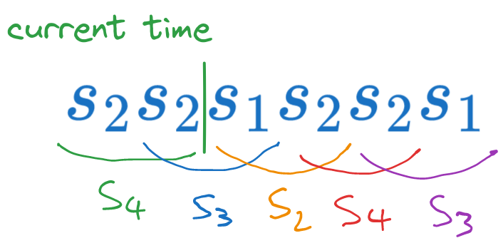
This is an extension of the previous question. We start in state \(S_4\), generating \(s_1\) will move to state \(S_3\), then generating \(s_2\) will move to state \(S_2\), then generating \(s_2\) moves to state \(S_4\), and finally generating \(s_1\) moves to state \(S_3\). Thus we go through the sequence of states \(S_4 \rightarrow S_3 \rightarrow S_2 \rightarrow S_4 \rightarrow S_3\).

Fig. 4.5 Sequence of states when generating \(s_1 s_2 s_2 s_1\) from state \(S_4\)

Each transition has a probability, found in the transition matrix, and we multiply them together to obtain the probability of the chain:

\[\begin{split} \begin{aligned} P &= P(S_4 \rightarrow S_3) \cdot P(S_3 \rightarrow S_2) \cdot P(S_2 \rightarrow S_4) \cdot P(S_4 \rightarrow S_3) \\ &= P(S_3|S_4) \cdot P(S_2|S_3) \cdot P(S_4|S_2) \cdot P(S_3|S_4) \\ &= \frac{1}{2} \cdot \frac{3}{8} \cdot \frac{3}{4} \cdot \frac{1}{2} \\ &= \frac{9}{128} \end{aligned} \end{split}\]

f. Compute the entropy in state \(S_4\);

In state \(S_4\), the probabilities are the ones in the 4th row of the transition matrix. There are only two messages which can be generated, \(s_1\) and \(s_2\), but the other two zeros do no harm anyway to the entropy.

\[ [0 \quad 0 \quad \frac{1}{2} \quad \frac{1}{2}\ \]

The entropy in state \(S_4\) is therefore the entropy computed for this distribution:

\[ H(S_4) = - \frac{1}{2} \log_2 \frac{1}{2} - \frac{1}{2} \log_2 \frac{1}{2} = 1 \, \text{bit} \]

g. Compute the global entropy of the source;

First we compute the entropy in every state, then we compute the stationary probabilities, and then we compute the average.

The entropy in every state is:

\[\begin{split} \begin{aligned} H(S_1) &= - \frac{1}{2} \log_2 \frac{1}{2} - \frac{1}{2} \log_2 \frac{1}{2} = 1 \, \text{bit} \\ H(S_2) &= - \frac{1}{4} \log_2 \frac{1}{4} - \frac{3}{4} \log_2 \frac{3}{4} = 0.8113 \, \text{bits} \\ H(S_3) &= - \frac{5}{8} \log_2 \frac{5}{8} - \frac{3}{8} \log_2 \frac{3}{8} = 0.9544 \, \text{bits} \\ H(S_4) &= - \frac{1}{2} \log_2 \frac{1}{2} - \frac{1}{2} \log_2 \frac{1}{2} = 1 \, \text{bit} \end{aligned} \end{split}\]

Next, we compute the stationary probabilities from the system:

\[ [p_1, p_2, ... p_N] \cdot [T] = [p_1, p_2, ... p_N] \]

which, in our case, means the following system of equations, written either in matrix form or as separate equations:

\[\begin{split} [p_1 \quad p_2 \quad p_3 \quad p_4] \cdot \begin{bmatrix} \frac{1}{2} & \frac{1}{2} & 0 & 0 \\ 0 & 0 & \frac{1}{4} & \frac{3}{4} \\ \frac{5}{8} & \frac{3}{8} & 0 & 0 \\ 0 & 0 & \frac{1}{2} & \frac{1}{2} \end{bmatrix} = \begin{bmatrix} p_1 \quad p_2 \quad p_3 \quad p_4 \end{bmatrix} \end{split}\]

i.e.:

\[\begin{split} \begin{cases} \frac{1}{2}p_1 + \frac{5}{8} p_3 &= p_1 \\ \frac{1}{2}p_1 + \frac{3}{8} p_3 &= p_2 \\ \frac{1}{4}p_2 + \frac{1}{2} p_4 &= p_3 \\ \frac{3}{4}p_2 + \frac{1}{2} p_4 &= p_4 \end{cases} \end{split}\]

However, this is not a linear independent system, and one equation is dependent on the others. Therefore, we eliminate one of the equations (any one, which ever looks harder), and we replace it with \(p_1 + p_2 + p_3 + p_4 = 1\).

Eliminating the second equation in the system results in:

\[\begin{split} \begin{cases} \frac{1}{2}p_1 + \frac{5}{8} p_3 &= p_1 \\ \sout{ \frac{1}{2}p_1 + \frac{3}{8} p_3} &\sout{= p_2} \\ \frac{1}{4}p_2 + \frac{1}{2} p_4 &= p_3 \\ \frac{3}{4}p_2 + \frac{1}{2} p_4 &= p_4 \\ p_1 + p_2 + p_3 + p_4 &= 1 \end{cases} \end{split}\]

Solving this system through any method gives the stationary probabilities:

\[\begin{split} \begin{aligned} p_1 &= ... \\ p_2 &= ... \\ p_3 &= ... \\ p_4 &= ... \end{aligned} \end{split}\]

Finally, we compute the global entropy of the source as the average of the state entropies, weighted by the stationary probabilities:

\[\begin{split} \begin{aligned} H(S) &= p_1 H(S_1) + p_2 H(S_2) + p_3 H(S_3) + p_4 H(S_4) \\ &= \dots \end{aligned} \end{split}\]

h. If the source is initially in state \(S_2\), in what states and with what probabilities will the source be after 2 messages?

We use the general formula which gives the probabilities at time \((n+1)\) based on the probabilities at time \(n\):

\[ [p_1^{(n)}, p_2^{(n)}, ... , p_N^{(n)}] \cdot [T] = [p_1^{(n+1)}, p_2^{(n+1)}, ... , p_N^{(n+1)}] \]

In our case, the initial probabilities are \([0, 1, 0, 0]\), because we are told the source is initially in state \(S_2\). After 2 messages, it means we multiply twice with \([T]\):

\[ \begin{bmatrix} 0 & 1 & 0 & 0 \end{bmatrix} \cdot [T] \cdot [T]= [p_1^{(2)}, p_2^{(2)}, p_3^{(2)}, p_4^{(2)}] \]

Therefore we have:

\[\begin{split} \begin{aligned} [p_1^{(2)}, p_2^{(2)}, p_3^{(2)}, p_4^{(2)}] &= \begin{bmatrix} 0 & 1 & 0 & 0 \end{bmatrix} \begin{bmatrix} \frac{1}{2} & \frac{1}{2} & 0 & 0 \\ 0 & 0 & \frac{1}{4} & \frac{3}{4} \\ \frac{5}{8} & \frac{3}{8} & 0 & 0 \\ 0 & 0 & \frac{1}{2} & \frac{1}{2} \end{bmatrix} \begin{bmatrix} \frac{1}{2} & \frac{1}{2} & 0 & 0 \\ 0 & 0 & \frac{1}{4} & \frac{3}{4} \\ \frac{5}{8} & \frac{3}{8} & 0 & 0 \\ 0 & 0 & \frac{1}{2} & \frac{1}{2} \end{bmatrix}\\ &= \begin{bmatrix} 0 & 0 & \frac{1}{4} & \frac{3}{4} \end{bmatrix} \begin{bmatrix} \frac{1}{2} & \frac{1}{2} & 0 & 0 \\ 0 & 0 & \frac{1}{4} & \frac{3}{4} \\ \frac{5}{8} & \frac{3}{8} & 0 & 0 \\ 0 & 0 & \frac{1}{2} & \frac{1}{2} \end{bmatrix}\\ &= \begin{bmatrix} \frac{5}{32} & \frac{3}{32} & \frac{3}{8} & \frac{3}{8} \end{bmatrix} \end{aligned} \end{split}\]

The most likely state in which the source will be after 2 messages is \(S_3\) or \(S_4\), and the least likely state is \(S_2\).