5. Source Coding

5.1. Exercise 1

Consider the binary codes below:

Message	Code A	Code B	Code C	Code D	Code E	Code F
\(s_1\)	\(00\)	\(0\)	\(0\)	\(0\)	\(0\)	\(0\)
\(s_2\)	\(01\)	\(10\)	\(01\)	\(100\)	\(110\)	\(10\)
\(s_3\)	\(10\)	\(110\)	\(011\)	\(11\)	\(10\)	\(11\)
\(s_4\)	\(11\)	\(1110\)	\(0111\)	\(110\)	\(111\)	\(110\)

For each code:

• a). Verify the Kraft inequality

• b). Determine if the code is instantaneous / uniquely decodable

• c). Draw the graph

5.1.1. Solution

Let’s analyze a) and b) for each code.

The Kraft inequality is:

\[\sum_{i=1}^{n} 2^{-l_i} \leq 1\]

where \(l_i\) is the length of the \(i\)-th codeword.

Code A. For the first codeword, all 4 codewords have length 2, so the sum is:

\[2^{-2} + 2^{-2} + 2^{-2} + 2^{-2} = 4 \cdot 2^{-2} = 1 (OK)\]

The code is instaneaneous because no codeword is a prefix of another codeword. This means it is also uniquely decodable.

Code B. For the second codeword the lengths are 1, 2, 3, 4, so the sum is:

\[2^{-1} + 2^{-2} + 2^{-3} + 2^{-4} = 1/2 + 1/4 + 1/8 + 1/16 = 15/16 < 1 (OK)\]

The code is instaneaneous, so it is uniquely decodable.

Code C. For the third codeword the lengths are also 1, 2, 3, 4 so the sum is the same as before.

The code is not instantaneous because the codeword for \(s_1\) is a prefix of all the other codewods. However, the code is uniquely decodable, because of the following argument: each 0 marks the begining of a codeword, so given any binary sequence there will be no problem splitting it into codewords, because we just have to look for the 0s.

Code D. For the fourth codeword the lengths are 1, 3, 2, 3, so the sum is:

\[2^{-1} + 2^{-3} + 2^{-2} + 2^{-3} = 1/2 + 1/8 + 1/4 + 1/8 = 1 (OK)\]

The code is not instantaneous because the codeword for \(s_3\) is a prefix of the codeword for \(s_4\). It is also not uniquely decodable, because of the following argument: given the sequence 110, we can’t tell if it is \(s_4\) or \(s_3 s_1\).

Code E. For the fifth codeword the lengths are also 1, 3, 2, 3, so the sum is the same as before.

The code is instantaneous, so it is uniquely decodable.

Code F. For the sixth codeword the lengths are 1, 2, 2, 2, so the sum is:

\[2^{-1} + 2^{-2} + 2^{-2} + 2^{-2} = 1/2 + 1/4 + 1/4 + 1/4 > 1 (BAD)\]

The code is not instantaneous nor uniquely decodable, because no code with these four lenghts can ever be, since the Kraft inequality is violated.

c). The graphs for the codes are represened below.

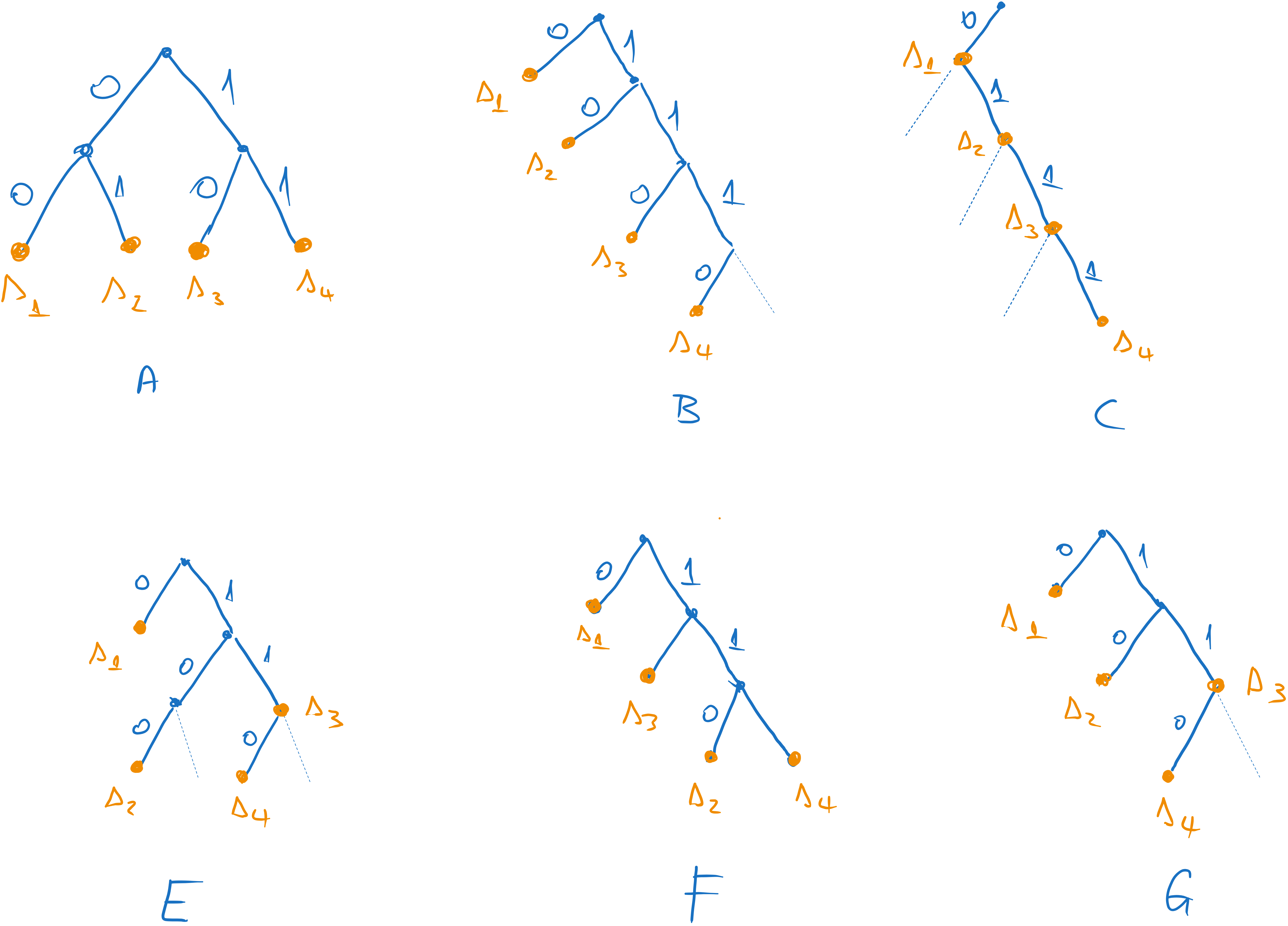
Fig. 5.1 The graphs of the codes A, B, C, D, E, and F.

5.2. Exercise 2

Consider a memoryless source with the following distribution:

\[ \sIV{S}{\frac{1}{2}}{\frac{1}{4}}{\frac{1}{8}}{\frac{1}{8}} \]

For this source we use two separate codes:

Message	Code A	Code B
\(s_1\)	\(00\)	\(0\)
\(s_2\)	\(01\)	\(10\)
\(s_3\)	\(10\)	\(110\)
\(s_4\)	\(11\)	\(111\)

Requirements:

• a). Compute the average lengths of the two codes

• b). Compute the efficienty and redundancy of the two codes

• c). Encode the sequence \(s_2s_4s_3s_3s_1\) with each code

• d). Decode the sequence 011010101010111100001010 with each code

5.2.1. Solution

a) Compute the average lengths of the two codes

The average length of a code is given by:

\[L = \sum_{i=1}^{n} p_i l_i\]

where \(p_i\) is the probability of the \(i\)-th message and \(l_i\) is the length of the codeword for the \(i\)-th message.

For Code A, we have:

\[\overline{l}_A = \frac{1}{2} \cdot 2 + \frac{1}{4} \cdot 2 + \frac{1}{8} \cdot 2 + \frac{1}{8} \cdot 2 = 2\]

For Code B, we have:

\[\overline{l}_B = \frac{1}{2} \cdot 1 + \frac{1}{4} \cdot 2 + \frac{1}{8} \cdot 3 + \frac{1}{8} \cdot 3 = 1.75\]

b) Compute the efficienty and redundancy of the two codes

We need first to compute the entropy of the source.

\[ H_A(S) = -\frac{1}{2} \log_2(\frac{1}{2}) -\frac{1}{4} \log_2(\frac{1}{4}) - 2 \cdot \frac{1}{8} \log_2(\frac{1}{8}) = 1.75 \]

Therefore the efficiency of Code A is \(\eta_A = H(S) / \overline{l}_A = 1.75 / 2 = 0.875\), and the (relative) redundancy is \(\rho_A = 1 - \eta_A = 0.125\).

For Code B, \(\eta_B = 1.75 / 1.75 = 1\) and \(\rho_B = 0\).

c) Encode the sequence \(s_2s_4s_3s_3s_1\) with each code

We just replace the messages with their codewords, according to each code.

With Code A we get:

\[ 0111101000 \]

With Code B:

\[ 101111101100 \]

d) Decode the sequence 011010101010111100001010 with each code

We need to identify the codewords in the sequence and replace them with the corresponding messages.

With Code A we get

\[ s_2 s_3 s_3 s_3 s_3 s_3 s_4 s_4 s_1 s_1 s_3 s_3 \]

Fig. 5.2 Decoding with the first code

With Code B we get:

\[ s_1 s_3 s_2 s_2 s_2 s_2 s_4 s_2 s_1 s_1 s_1 s_2 s_2 \]

Fig. 5.3 Decoding with the second code

5.3. Exercise 3

Fill in the missing bits (marked with ?) such that the resulting code is instantaneous.

Message	Codeword
\(s_1\)	\(??\)
\(s_2\)	\(1??\)
\(s_3\)	\(11?\)
\(s_4\)	\(0?\)
\(s_5\)	\(??\)

(just replace the ‘?’; do not add additional bits)

5.3.1. Solution

This is a creative exercise. We don’t have a fixed algorithm to solve it, but we can try to find a solution by trial and error. Note that since the code is instantaneous, no codeword can be a prefix of another codeword.

For example, we observe that we have three codewords with lengths 2, which will occupy three quarters of the graph. This means that the codewords for \(s_2\) and \(s_3\), which have length 3, must both stem from the same node (have the same two bits). Thus, we can choose:

\[\begin{split} s_3 = 111 \\ s_2 = 110 \end{split}\]

The other codewords occupy all other combinations of two bits (\(00\), \(01\), \(10\)), for example:

\[\begin{split} s_1 = 00 \\ s_4 = 01 \\ s_5 = 10 \end{split}\]

5.4. Exercise 4

We perform Shannon coding on an information source with \(H(S) = 20\)b.

• a. What are the possible values for the efficiency of the code?

• b. What are the possible values for the redundancy of the code?

• c. What is the minimum number of messages the source may possibly have?

5.4.1. Solution

a. What are the possible values for the efficiency of the code?

We know that if we do Shannon coding, the average length of the resulting code is between \(H(S)\) and \(H(S) + 1\):

\[ H(S) \leq \overline{l} < H(S) + 1 \]

This means the efficiency, which is \(\overline{l} / H(S)\), is between:

\[ \frac{H(S)}{H(S)+1} < \eta \leq 1 \]

which means \(\eta \in (0.95, 1]\)

b. What are the possible values for the redundancy of the code?

The relative redundancy is \(\rho = 1 - \eta\), so it is between 0 and 0.05.

The absolute redundancy is \(R = H(S) - \overline{l}\), so it is between 0 and 1.

5.4.2. c. What is the minimum number of messages the source may possibly have?

Because the entropy of the source is 20 bits, this means the source has many messages.

Remember one of the properties of entropy, that it is maximum when all messages are equally probable, and in this case the entropy is \(\log_2(n)\), where \(n\) is the number of messages:

\[ H_{max} = \log_2(n) \]

Out source has an entropy of \(H(S) = 20\) bits, so the maximum entropy is at least 20 bits. We have:

\[ 20 \leq \log_2(n) \]

which means \(n \geq 2^{20}\), so the source must have at least \(2^{20} = 1048576\) messages in order to be possible to have an entropy of 20 bits.

5.5. Exercise 5

A discrete memoryless source has the following distribution:

\[\sV{S}{0.05}{0.4}{0.1}{0.25}{0.2}\]

• a. Encode the source with Shannon, Shannon-Fano coding and Huffman coding and compute the average length in every case.

• b. Find the efficiency and redundancy of the Huffman code

• c. Compute the probabilities of the symbols \(0\) and \(1\), for the Huffman code

5.5.1. Solution

a. Encode the source with Shannon, Shannon-Fano coding and Huffman coding and compute the average length in every case

The three coding methods are explained below.

Shannon encoding:

1. We arrange the probabilities in descending order:

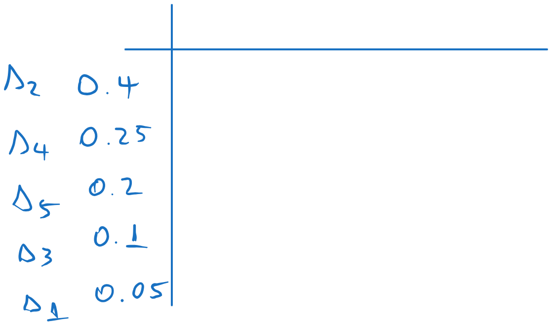
2. We compute the codeword lenghts with \(l_i = \lceil -\log_2(p_i) \rceil\), where \(\lceil \cdot \rceil\) means “rounding upwards”:

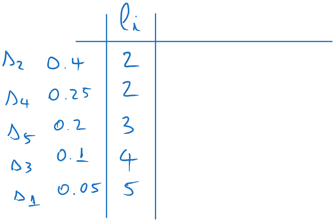
3. We compute the cumulative sum probabilities, i.e. the sum of the probabilities up to the current row, but not including the current row:

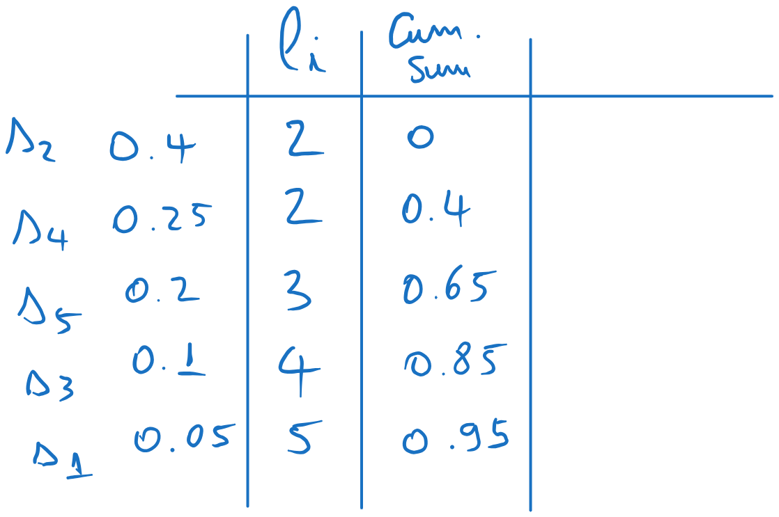
4. We find the codewords as follows, adding another three columns:

   4.1 Compute the values \(\lfloor cumsum \cdot 2^l_i \rfloor\) (the cumulative values multiplied by \(2^{l_i}\), rounded downwards). 4.2 Write these values in binary, using \(l_i\) bits. If there are less bits than \(l_i\), add zeros to the left. These are the codewords,

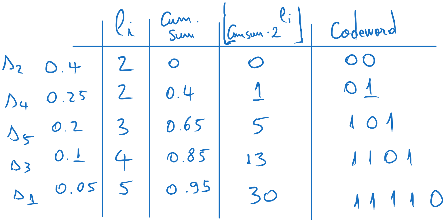
Fig. 5.4 Obtaining the codewords using Shannon coding

Shannon-Fano coding:

1. We arrange the probabilities in descending order:

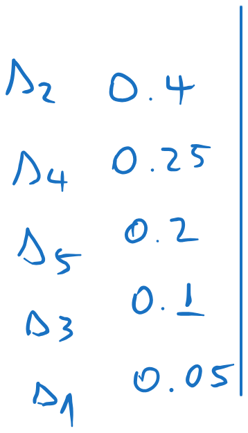
2. We split the list in two, such that the sum of the probabilities in each part is as close as possible (i.e. as close as possible to \((0.5, 0.5)\)). We assign 0 to one part and 1 to the other.

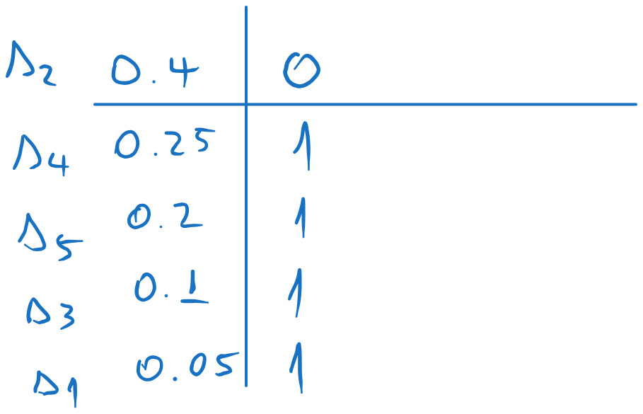
3. We repeat the process for each sub-list, splitting each in two as close as possible and assigning 0 and 1 to each sub-part.

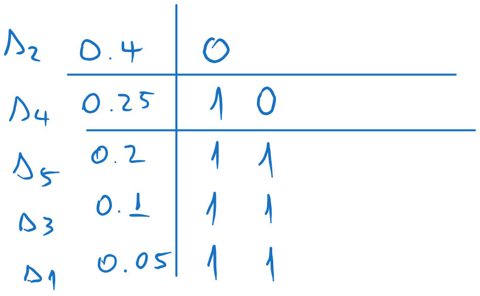
4. We continue until we have only one element in each sub-list. Each element will have the corresponding codeword.

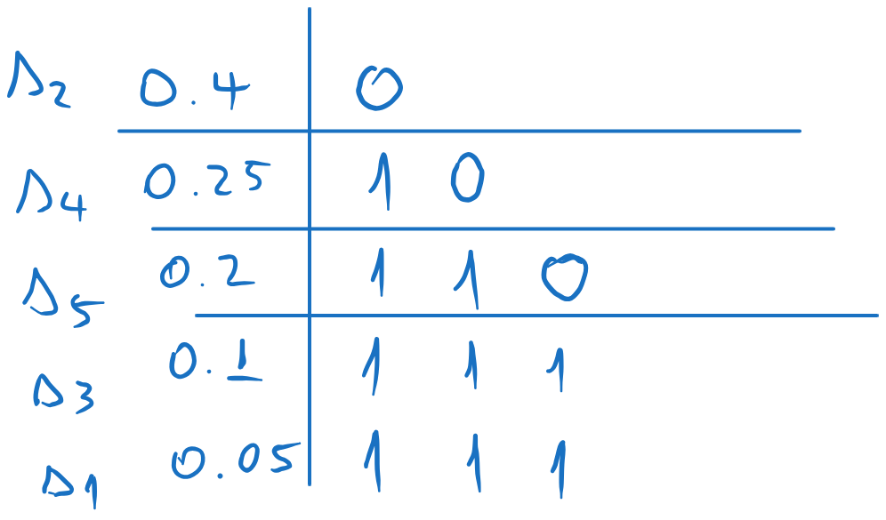
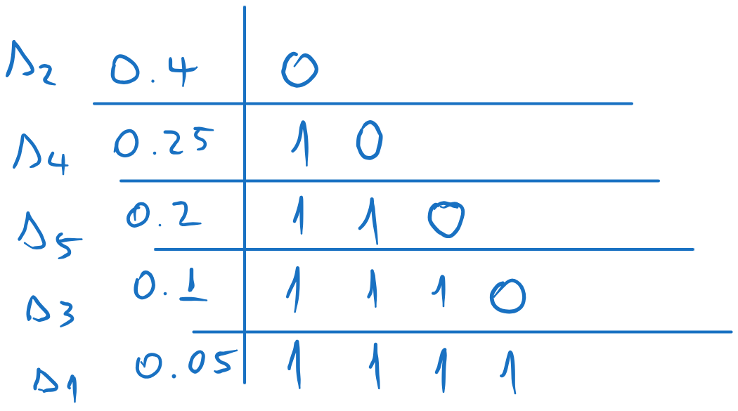
Fig. 5.5 Codewords obtained with Shannon-Fano coding

Huffman coding:

1. We arrange the probabilities in descending order:

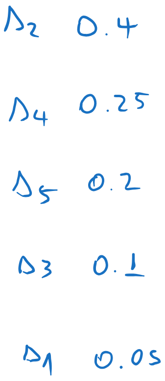
2. We sum the messages with the lowest probabilities, and we insert the sum in the list, keeping the list sorted. All other messages are kept in the same order. In this case, the combined message ends at the bottom of the list.

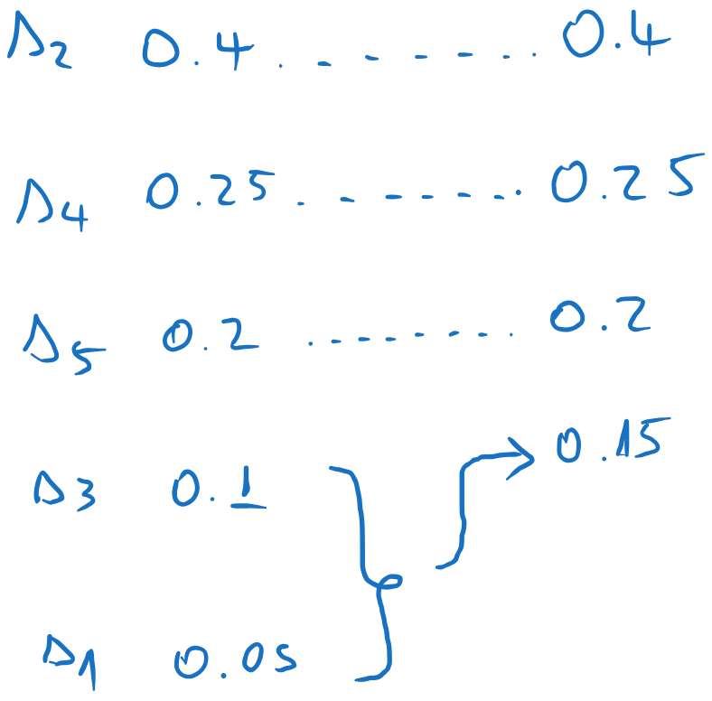
3. We repeat the process until we have just two elements. Every time we add the last two elements, and we insert the result among the other elements, keeping the list sorted.

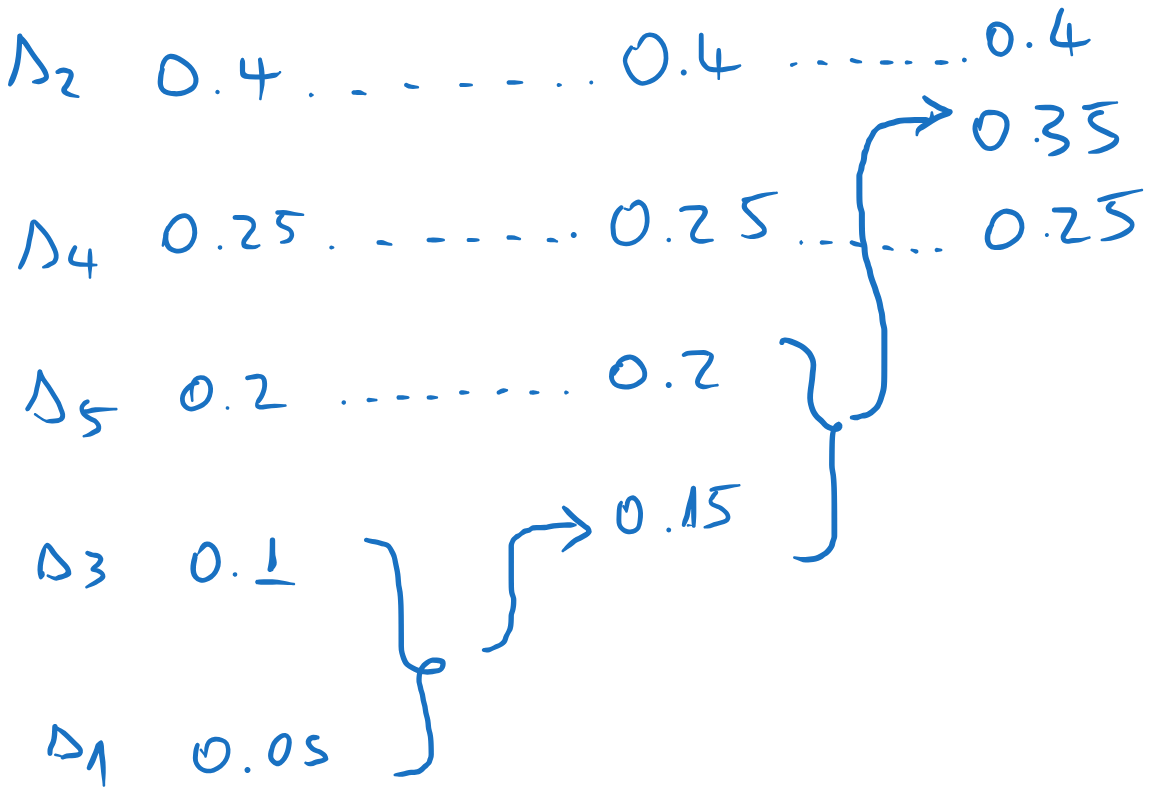
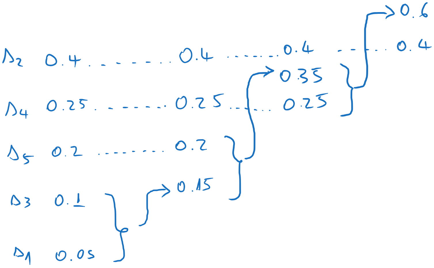
4. Now we start the backward pass. We assign 0 and 1 to the final two messages

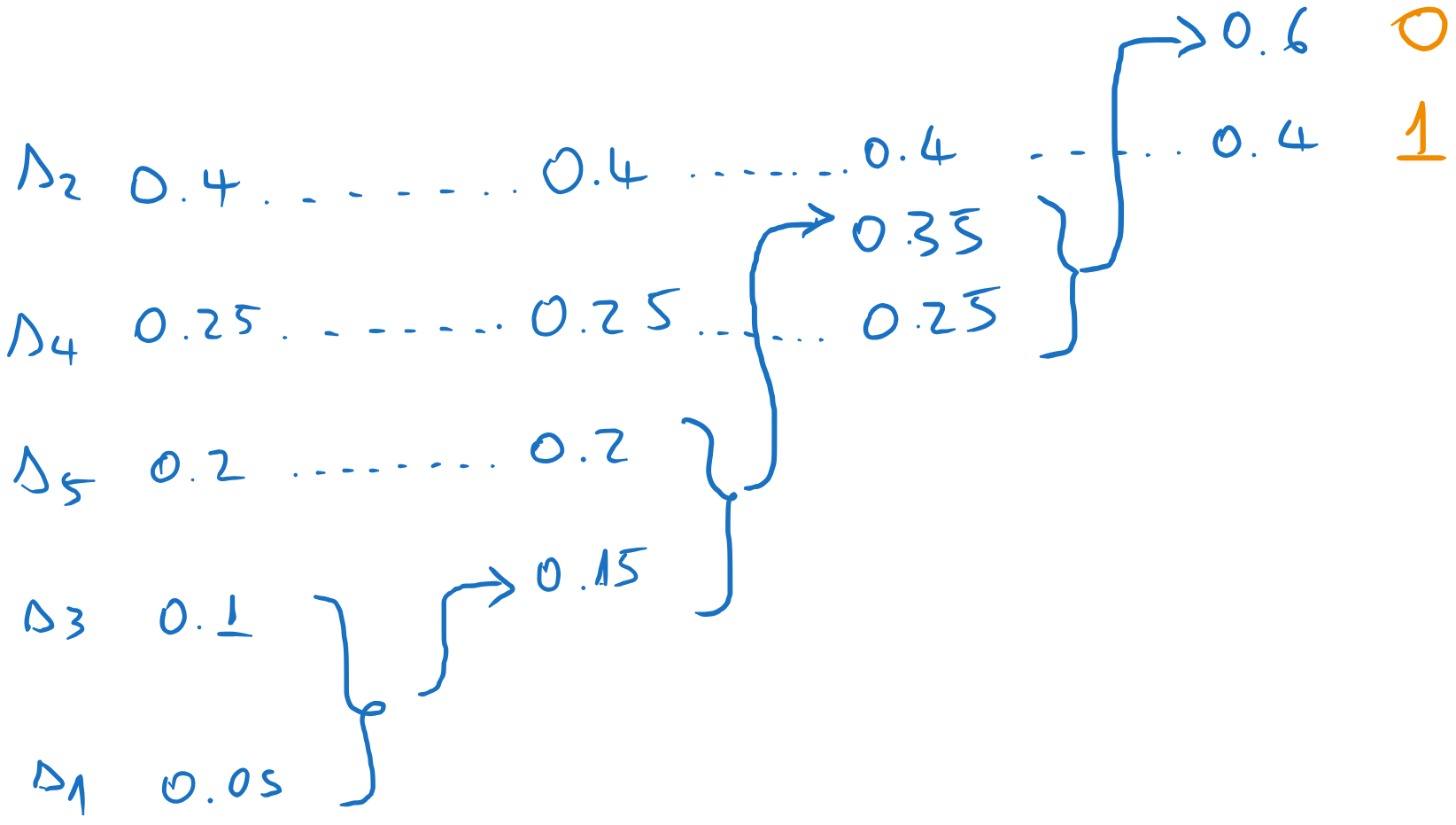
5. We go one column to the left, and we assign codewords to the two messages which were combined in the previous step. The codewords inherit the codeword of the parent (0), to which we append an extra 0 and 1.

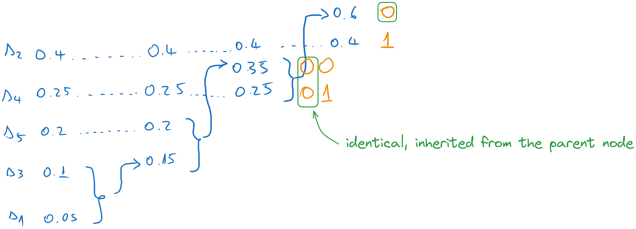
6. We continue until we reach the first column. Every time we take the codeword of the parent and we append a 0 and a 1 to form the codewords of the combined messages. All other messages just inherit the previous codeword.

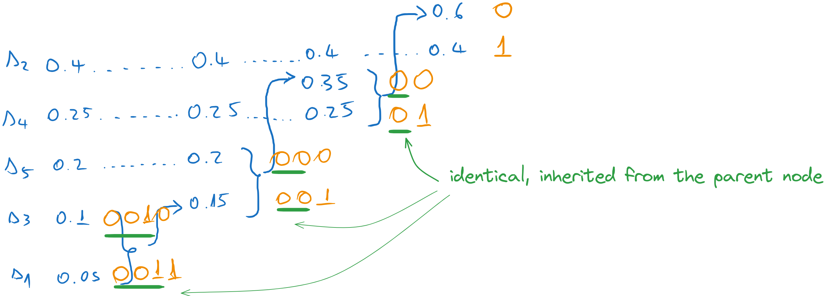
7. In the end, we read the codewords of each message along the lines.

Fig. 5.6 Codewords obtained with Huffman coding

Once we have the codewords, we can compute the average length of the code:

\[ \overline{l} = \sum_{i=1}^{n} p_i l_i \]

where \(p_i\) is the probability of the \(i\)-th message and \(l_i\) is the length of the codeword for the \(i\)-th message.

For the Shannon code, we have:

\[ \overline{l}_S = 0.05 \cdot 5 + 0.4 \cdot 2 + 0.1 \cdot 4 + 0.25 \cdot 2 + 0.2 \cdot 3 = 2.45 \text{ bits} \]

For the Shannon-Fano code, we have:

\[ \overline{l}_F = 0.05 \cdot 4 + 0.4 \cdot 1 + 0.1 \cdot 4 + 0.25 \cdot 2 + 0.2 \cdot 3 = 2.1 \text{ bits} \]

For the Huffman code, we have:

\[ \overline{l}_H = 0.05 \cdot 4 + 0.4 \cdot 1 + 0.1 \cdot 4 + 0.25 \cdot 2 + 0.2 \cdot 3 = 2.1 \text{ bits} \]

b) Find the efficiency and redundancy of the Huffman code

We need first to compute the entropy of the source.

\[ H(S) = -0.05 \log_2(0.05) - 0.4 \log_2(0.4) - 0.1 \log_2(0.1) - 0.25 \log_2(0.25) - 0.2 \log_2(0.2) = 2.04 \text{ bits} \]

The efficiency of the Huffman code is

\[ \eta = \frac{H(S)}{\overline{l}_H} = \frac{2.04}{2.1} = 0.971$ \]

The relative redundancy is \(\rho = 1 - \eta = 0.029\), and the absolute redundancy is \(R = \overline{l}_H - H(S) = 0.06\) bits.

c) Compute the probabilities of the symbols \(0\) and \(1\), for the Huffman code

We need first to compute the average numbers of 0’s and average number of 1’s in the codewords, \(\overline{l}_0\) and \(\overline{l}_1\). We compute them just like the average length, but we consider only the number of 0’s and 1’s in the codewords, not the full codeword lenghts.

We have:

\[ \overline{l}_0 = 0.05 \cdot 2 + 0.4 \cdot 0 + 0.1 \cdot 3 + 0.25 \cdot 1 + 0.2 \cdot 3 = 1.25 \text{ bits} \]

\[ \overline{l}_1 = 0.05 \cdot 2 + 0.4 \cdot 1 + 0.1 \cdot 1 + 0.25 \cdot 1 + 0.2 \cdot 0 = 0.85 \text{ bits} \]

Note that \(\overline{l}_0 + \overline{l}_1 = \overline{l}_H\).

The probabilities of 0 and 1 are:

\[ p_0 = \frac{\overline{l}_1}{\overline{l}} = \frac{1.25}{2.1} = 0.595 \]

\[ p_1 = \frac{\overline{l}_0}{\overline{l}} = \frac{0.85}{2.1} = 0.405 \]

This means that 0’s predominates in the codewords.

5.6. Exercise 6

For the following source, perform Huffman coding and obtain two different codes with same average length, but different individual codeword length.

\[\sVI{S}{0.05}{0.05}{0.15}{0.25}{0.25}{0.25}\]

Compute the average length in all three cases and show it is the same.

5.6.1. Solution

Huffman codes with the same average length but different individual codeword lengths are obtained when the sum of the probabilities of the two least probable messages is the same as some other values in the list, such that we can place the result in different positions in the list.

Let us start Huffman coding on this source. At the second step, we obtain a combined message with probability \(0.25\), which could be inserted in several positions in the list.

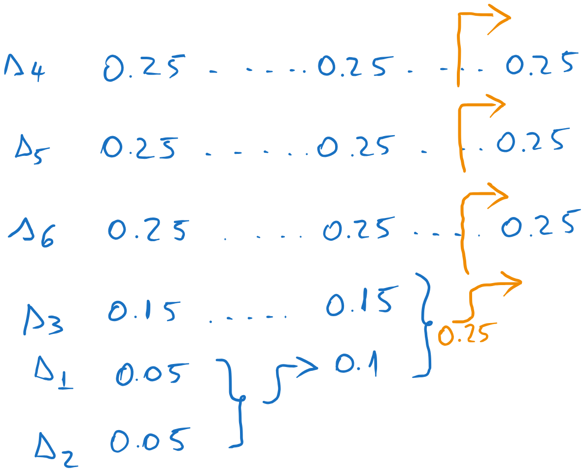
Fig. 5.7 Different placement options.

Each of the four options will lead to a slightly different code, but with the same average length, but with possibly different individual codeword lengths.

Let us proceed with three different cases and compute the average length in each case.

Variant 1

Suppose we choose the lowest position for the combined message. Continuing the process, we obtain the following codewords:

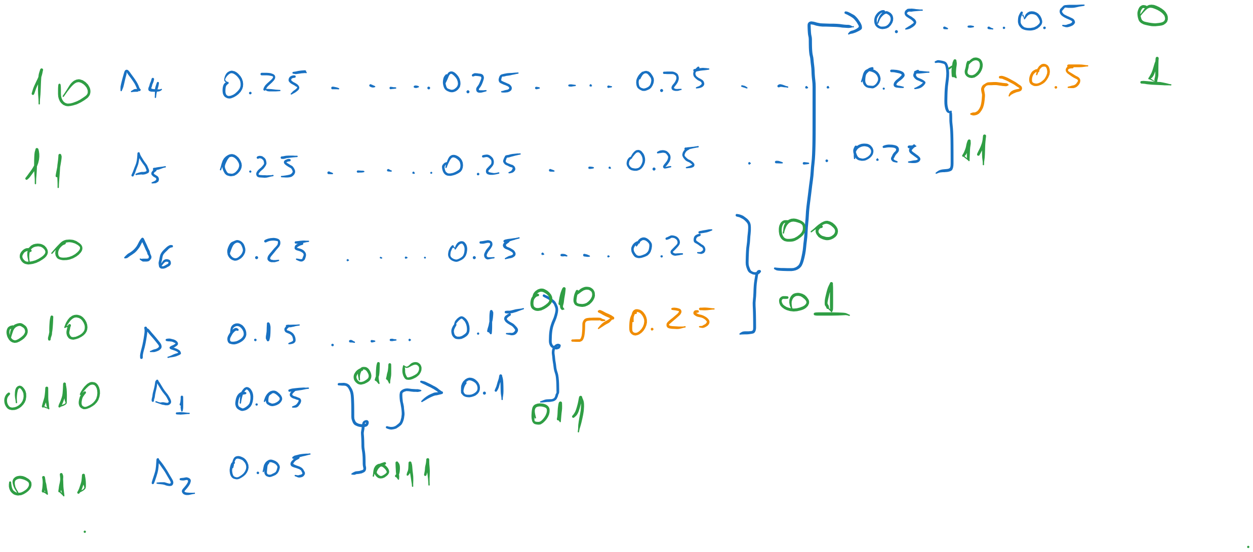
Fig. 5.8 Codewords for the first variant.

Note that we also had another option to choose for the \(0.5\) value, but this one has little impact on the final result, because it is close to the end.

The average codeword length is:

\[ \overline{l}_1 = 0.05 \cdot 4 + 0.05 \cdot 4 + 0.15 \cdot 3 + 0.25 \cdot 2 + 0.25 \cdot 2 + 0.25 \cdot 2 = 1.6 \]

Variant 2

Suppose we choose instead the highest position for the combined message. We obtain:

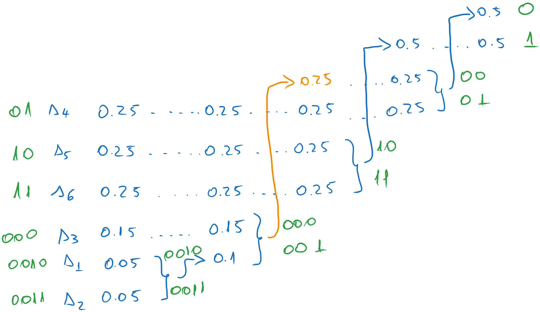
Fig. 5.9 Codewords for the second variant.

In fact, the codeword lengths are the same as in the previous case, because the list of messages is small. If we had an example with many more messages, the codeword lengths would have been different.

The average codeword length is the same:

\[ \overline{l}_2 = 0.05 \cdot 4 + 0.05 \cdot 4 + 0.15 \cdot 3 + 0.25 \cdot 2 + 0.25 \cdot 2 + 0.25 \cdot 2 = 1.6 \]

5.7. Exercise 7

A discrete memoryless source has the following distribution:

\[\sIII{S}{0.1}{0.7}{0.2}\]

• a). Find the average code length obtained with Huffman coding on the original source and on its second order extension.

• b). Encode the sequence \(s_2 s_2 s_3 s_2 s_2 s_2 s_1 s_3 s_2 s_2\) with both codes.

5.7.1. Solution

a). Find the average code length obtained with Huffman coding on the original source and on its second order extension.

For the original source, we have the following coding process:

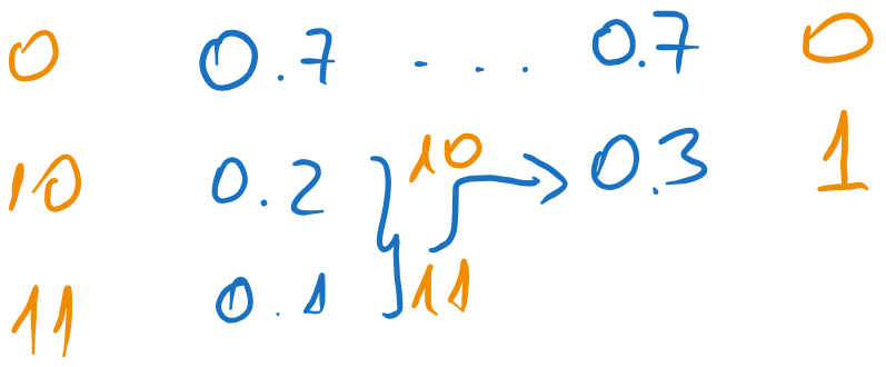
Fig. 5.10 Huffman coding of the original source

The average length is:

\[ \overline{l}_1 = 0.1 \cdot 2 + 0.7 \cdot 1 + 0.2 \cdot 2 = 1.3 \]

The second order extension is obtained by considering all possible pairs of messages:

\[\begin{split} S^2: \left( \begin{matrix} s_1s_1 & s_1s_2 & s_1s_3 & s_2s_1 & s_2s_2 & s_2s_3 & s_3s_1 & s_3s_2 & s_3s_3 \\ 0.01 & 0.07 & 0.02 & 0.07 & 0.49 & 0.14 & 0.02 & 0.14 & 0.04 \end{matrix} \right) \end{split}\]

The Huffman coding is:

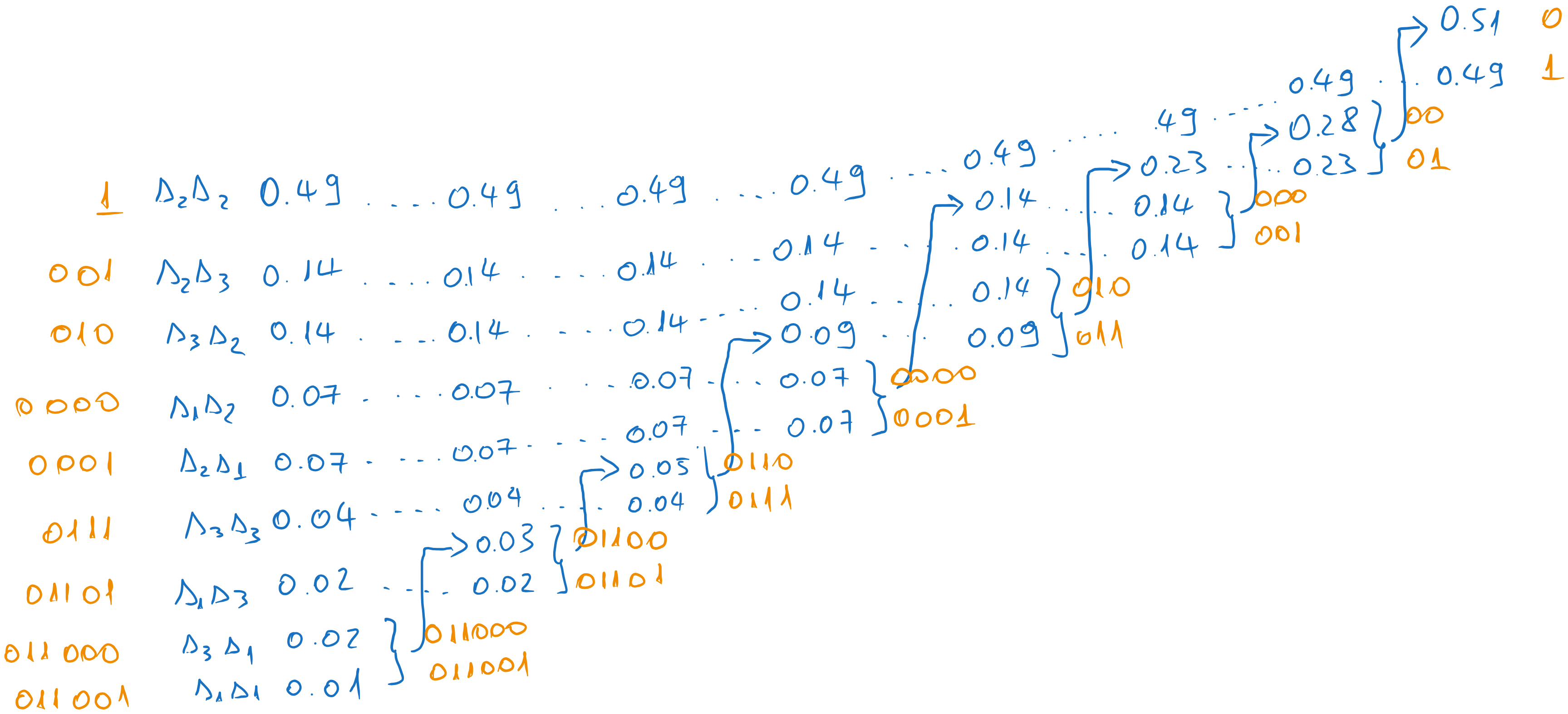
Fig. 5.11 Huffman coding of the second order extension

The average length is:

\[\begin{split} \begin{align*} \overline{l}_2 &= 0.01 \cdot 6 + 0.07 \cdot 4 + 0.02 \cdot 5 + 0.07 \cdot 4 + 0.49 \cdot 1 + 0.14 \cdot 3 + 0.02 \cdot 6 + 0.14 \cdot 3 + 0.04 \cdot 4 = \\ &= 2.33 \end{align*} \end{split}\]

Note that the second order extension is more efficient than the first, because it is better to encode a pair of messages with \(2.33\) bits on average than each message with \(1.3\) bits on average.

b). Encode the sequence \(s_2 s_2 s_3 s_2 s_2 s_2 s_1 s_3 s_2 s_2\) with both codes.

With the first code, we encode each individual message:

\[ 0010000111000 \]

With the second code, we encode each pair of messages with its codeword:

\[ 10101011011 \]

5.8. Exercise 8

A discrete memoryless source has the following distribution

\[\sVIII{S}{0.4}{0.3}{0.2}{0.04}{0.03}{0.02}{0.009}{0.001}\]

Find the Huffman code for a code with 4 symbols, \(x_1\), \(x_2\), \(x_3\) and \(x_4\), and encode the following sequence:

\[ s_1 s_7 s_8 s_3 s_3 s_1 \]

5.8.1. Solution

For the Huffman code with 4 symbols, we combine the last 4 messages in the list.

Note

We need to add two virtual messages (of probability 0) to the initial list, such that number of messages remaining in the last step is 4.

The Huffman coding proceeds as follows:

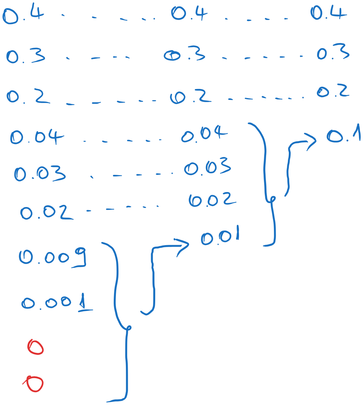
Fig. 5.12 Huffman coding of the source

At the backward pass, we assign the symbols \(x_1\), \(x_2\), \(x_3\) and \(x_4\) from right to left:

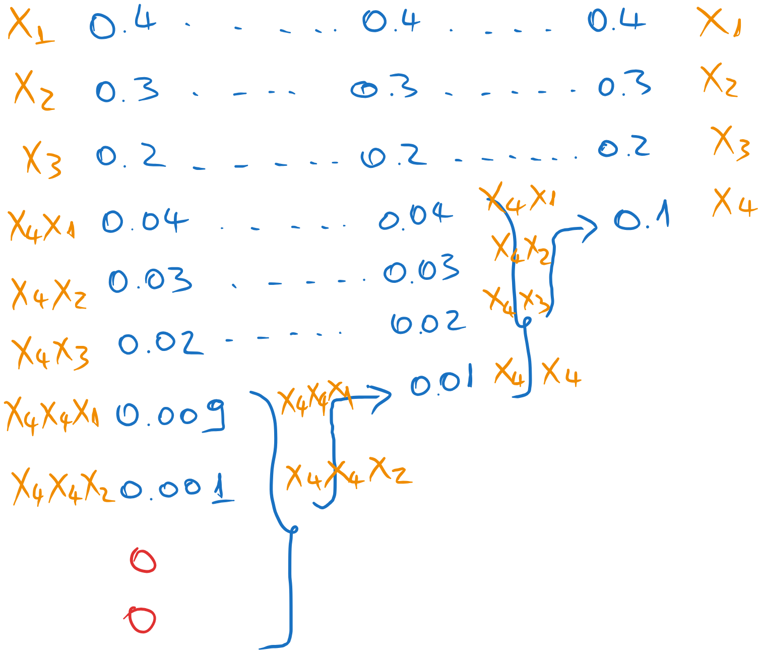
Fig. 5.13 Assigning the symbols

The average length of the code is:

\[ \overline{l} = 0.4 \cdot 1 + 0.3 \cdot 1 + 0.2 \cdot 1 + 0.04 \cdot 2 + 0.03 \cdot 2 + 0.02 \cdot 2 + 0.009 \cdot 3 + 0.001 \cdot 3 = 1.11 \]

The sequence \(s_1 s_7 s_8 s_3 s_3 s_1\) is encoded as:

\[ x_1 x_4 x_4 x_1 x_4 x_4 x_2 x_3 x_3 x_1 \]