3 Digital filtering
In this chapter we discuss the filtering of digital signals, making use of the Fourier transform introduced in the previous chapter.
3.1 Transfer function of LTI systems
3.1.1 Response to complex exponentials
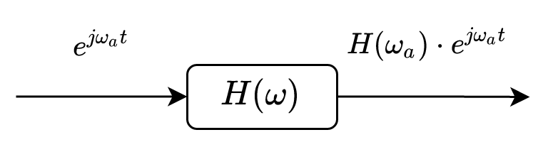
Let us consider a linear time-invariant (LTI) system with impulse response \(h[n]\). Let’s analyze the response of this system to harmonic signals.
First, let’s consider the input signal to be a complex exponential signal (we already saw this in the previous chapter, but we repeat it here for clarity):
\[x[n] = A e^{j \omega_0 n}\]
The output signal is obtained via convolution with the impulse response:
\[\begin{split} y[n] &= \sum_{k=-\infty}^\infty h[k] x[n-k]\\ &= \sum_{k=-\infty}^\infty h[k] e^{-j \omega_0 k} A e^{j \omega_0 n}\\ &= H(\omega_0) \cdot x[n] \end{split}\]
where \(H(\omega_0)\) is Fourier transform of \(h[n]\), \(H(\omega)\), evaluated for \(\omega = \omega_0\). Since \(H(\omega_0)\) is a complex value, with modulus and phase, this means the amplitude of the input gets multiplies by \(|H(\omega_0)|\), and the phase of the input signal is added with \(\angle H(\omega_0)\).
Complex exponential signals are eigen-functions (funcții proprii) of LTI systems, since the output is the input multiplied by a constant. - If input signal = sum of complex exponential (like coses + sinuses), - then output = same sum of complex exponentials, each scaled with some coefficients
A similar result holds for cosine and sine signals, since they can be written as sums of complex exponentials: \[\begin{split} \cos(\omega n) &= \frac{e^{j \omega n} + e^{-j \omega n}}{2}\\ \sin(\omega n) &= \frac{e^{j \omega n} - e^{-j \omega n}}{2j} \end{split}\]
3.1.2 Response to sinusoidal signals
If the input signal is a cosine (or a sine): \[x[n] = A \cos(\omega_0 n + \phi) = \frac{e^{j (\omega_0 n + \phi)} + e^{-j (\omega_0 n + \phi)}}{2}\] the output signal is: \[\begin{split} y[n] &= \frac{H(\omega_0) e^{j \omega_0 n + \phi} + H(-\omega_0) e^{-j \omega_0 n + \phi}}{2}\\ &= A |H(\omega_0)| \cos(\omega_0 n + \phi + \angle H(\omega_0)) \end{split}\] where we use the fact that \(H(-\omega_0) = H(\omega_0)^*\) (complex conjugate), since \(h[n]\) is real.
Similarly, the amplitude of the input signal is multiplied by \(|H(\omega_0)|\), and the phase of the input signal increases with \(\angle H(\omega_0)\).
3.1.3 Response to periodic signals
As an even more general case, consider an input \(x[n]\) which is periodic with period N. Then it can be represented as a Fourier series with coefficients \(X_k\): \[x[n] = \frac{1}{N} \sum_{k=0}^{N-1}X_k e^{j 2 \pi k n / N}\]
Since the system is linear, each component \(k\) gets multiplied with \(H\left(\frac{2 \pi}{N}k\right)\), so the output signal is: \[y[n] = \frac{1}{N}\sum_{k=0}^{N-1}X_k H\left(\frac{2 \pi}{N}k\right) e^{j 2 \pi k n / N}\]
The output signal \(y[n]\) is still periodic, with the same period, having the same frequencies, but each coefficient \(X_k\) is multiplied by \(H\left(\frac{2 \pi}{N}k\right)\), where \(k/N\) is the frequency of the \(k\)-th coefficient.
3.1.4 Response of LTI systems to non-periodic signals
Finally, let’s consider a general input \(x[n]\) (not periodic). The output signal is the convolution of the input signal with the impulse response: \[y[n] = x[n] * h[n]\] and, in the frequency domain, this corresponds to the product of the two DTFT transforms: \[Y(\omega) = X(\omega) \cdot H(\omega)\]
The transfer function \(H(\omega)\) “shapes” the input spectrum, in the same sense that the modulus of \(|H(\omega)|\) multiplies the modulus of the input spectrum \(|X(\omega)|\), while the phase of \(H(\omega)\) adds to the phase of \(X(\omega)\): \[\begin{split} |Y(\omega)| &= |X(\omega)| \cdot |H(\omega)|\\ \angle Y(\omega) &= \angle X(\omega) + \angle H(\omega) \end{split}\]
3.1.5 Transfer function
In all these cases we see that the system attenuates/amplifies the input frequencies and changes their phases, according to \(H(\omega)\).
The function \(H(\omega)\), which is the DTFT transform of \(h[n]\) \[H(\omega) = \sum_{n=-\infty}^\infty h[n] e^{-j \omega n}\] is called the transfer function of the system.
The system is also called a filter, because it filters the input signal by shaping its spectrum with the transfer function.
Remember that the function \(H(z)\), the Z transform of \(h[n]\), is called system function, and it is related to \(H(\omega)\) by \(H(z) = H(z=e^{j\omega})\) (if the unit circle is in the region of convergence).
The transfer function \(H(\omega)\) is also known as the frequency response of the system.
Its modulus \(|H(\omega)|\) is also known as the amplitude response of the system. Sometimes it is called the magnitude response, especially when the values are in decibels (dB).
Its phase \(\angle H(\omega)\) is also known as the phase response of the system.
- \(\angle H(\omega)\) = phase response
The amplitude response is always non-negative \(|H(\omega)| \geq 0\), while the phase response is an angle \(\angle H(\omega) \in (-\pi, \pi]\).
When working with filters, it is very common to plot the amplitude and phase responses, in order to understand how the filter shapes the input signal.
When considering phase reponse, the function may have jumps of \(2 \pi\) (known as wrapped phase), which has no practical meaning, but it makes the function discontinuous. It is common to unwrap the phase by eliminating these jumps in order to obtain a continuous function, which doesn’t mean any change in the actual phase of the signal, but produces a continuous function. The unwrapped phase can thus exceed the interval \((-\pi, \pi]\), while the wrapped phase is always in this interval.
TODO: example
3.2 Permanent and transient response
When working with filters, it is important to distinguish between the permanent and transient response of the system.
Let us consider applying an input signal \(\cos(\omega n)\) to a filter. It is true that the output signal is \[y[n] = |H(\omega)| \cos(\omega n + \angle H(\omega)),\] but this is valid only for the infinitely-long signal, which has been applied to the filter since \(n=-\infty\).
In practice, we apply the signal at some initial time \(n=0\). In fact, this means we’re not applying the true mathetmatical signal \(\cos(\omega n)\), but a portion of it. This means that the output signal will not be the same as the above formula, but it will have a transient response which will eventually vanish, leaving only the permanent response.
The permanent response is the response of the system after a very long time, when the transient response has vanished. Basically, we consider the starting time to be \(n=-\infty\), and the system has had enough time to reach the permanent response. In this case, we say the system is in permanent regime.
This formula is valid only in permanent regime: \[y[n] = |H(\omega)| \cos(\omega n + \angle H(\omega)),\] when the transient response has vanished.
Before reaching the permanent regime, the system is said to be in transient regime. In this regime, the output signal is not the same as the above formula, but it has a transient response which eventually vanishes: \[y[n] = |H(\omega)| \cos(\omega n + \angle H(\omega)) + \text{transient response}\]
The transient response goes towards 0 as \(n\) increases, while the permanent response remains.
3.3 Ideal filters, distortions, filter order
TODO: Draw the ideal transfer function of a:
- low-pass filter
- high-pass filter
- band-pass filter
- band-stop filter
- all-pass filter (changes the phase)
When a filter is non-ideal, this manifests as follows:
- The transfer function has a non-constant amplitude in the target frequency range. This leads to amplitude distortions.
- The transfer function has a non-linear phase in the target frequency range. This leads to phase distortions.
Note that thase distortions may be tolerated by certain applications, for example in audio processing, where the human ear is not very sensitive to phase distortions. However, in applications such as signal processing and communications, phase distortions are very important, since they distort the shape of the signal.
3.3.1 Filter order
The order of a filter is maximum degree in numerator or denominator of \(H(z)\), i.e. largest power of \(z\) or \(z^{-1}\) appearing in the transfer function. Also, it is the maximum number of poles or zeros of the filter.
Any filter can be implemented, in general, with this number of unit delay blocks (\(z^{-1}\)).
A filter with high order has a more complicated transfer function, since it has more coefficients in the numerator and denominator. As such, it can approximate better the ideal filter, but it is more complex to implement and has more delays.
A filter with low order has a simpler transfer function, but it cannot approximate an ideal filter as well. However, it is simpler to implement and has less delays.
3.4 Linear phase filters
3.4.1 EFfect of linear phase
A very important property of filters is the linearity of the phase response, i.e. the phase function is a linear function of the frequency: \[\angle H(\omega) = - \omega n_0\]
Let’s see what it means for a filter to have linear phase. Consider the following filter with linear phase function: \[\angle H(\omega) = -j \omega n_0,\] and, for simplicity, an amplitude response which is a constant \(C\): \[|H(\omega)| = C\] The transfer function is therefore: \[H(\omega) = C \cdot e^{- j \omega n_0}\]
For some input \(x[n]\), the output signal is: \[Y(\omega) = X(\omega) \cdot C \cdot e^{- j \omega n_0}\] which means \[y[n] = C \cdot x[n-n_0]\] since multiplying with \(e^{- j \omega n_0}\) in the frequency domain corresponds to a delay in the time domain: \[x[n-n_0] \leftrightarrow X(\omega) e^{-j \omega n_0}\]
We see, therefore, that linear phase means just delaying of the input signal. The slope of the phase response (\(n_0\)) is constant gives the amount of delay. Thus, a linear-phase filter just delays all frequencies with the same amount of time, without distorting the shape of signal.
Note that the phase response in in radians, and the delay is in samples (time). For a sinusoidal signal an extra phase of \(2 \pi\) means a delay of a period \(N = \frac{1}{f}\), therefore in order to delay all the frequencies with the same amount of time, the phase response must be a linear function of the frequency, such that the extra phase is linear with the frequency.
The group delay is the time delay experienced by a component of frequency \(\omega\) when passing through the filter, as opposed to the phase delay which is the phase added by the filter.
The group delay of the filter is defined as: \[\tau_g(\omega) = \frac{d \Theta(\omega)}{d \omega}\]
A linear-phase system means a constant group delay, which means that all frequency components are delayed with the same amount of time. This means that the whole signal is delayed, without distortions.
If a filter has a non-linear phase response, this means that the different frequency components are delayed with different amounts of time, which leads to distortions in the signal.
3.4.2 Conditions for linear phase
In order to have linear phase, a filter must satisfy certain symmetry cnoditions in the impulse response \(h[n]\).
A filter has linear phase if the impulse response has positive symmetry or negative symmetry around a central point \(n_0\), which is either an integer or a half-integer (\(x.5\) value).
First of all, let us state (without any proof) that, for causal systems, only FIR filters can have linear phase. Causal IIR filters cannot have linear phase. We will prove this statement later.
To clarify the symmetry conditions, let us consider a causal FIR filter with impulse response \(h[n]\) of length \(M\) (order \(M-1\)), i.e. the filter coefficients are \(h[0]\), \(h[1]\), …, \(h[M-1]\).
Linear phase is guaranteed in two cases:
Positive symmetry: \[h[n] = h[M-1-n]\]
Negative symmetry (anti-symmetry): \[h[n] = -h[M-1-n]\]
In both cases, the delay incurred by the linear phase is given by the middle point of the symmetry, e.g \(\frac{M-1}{2}\). If \(M\) is odd, the middle point is an integer (e.g. \(M=5\), coefficients go from \(h[0]\) to \(h[4]\), middle point is $n_0= 2 $). If \(M\) is even, the middle point is a half-integer (e.g. \(M=6\), coefficients go from \(h[0]\) to \(h[5]\), middle point is \(n_0 = 2.5\)).
In order to prove these conditions, we must consider all four scenarios:
- Positive symmetry, M = odd
- Positive symmetry, M = even
- Negative symmetry, M = odd
- Negative symmetry, M = even
3.4.2.1 Positive symmetry, M = odd
It is easier to start the proof from an example. Suppose we have a FIR filter with \(M=5\) coefficients: \[h[n] = \lbrace 4, 3, 2, 3, 4 \rbrace\] Its transfer function is: \[H(z) = 4 + 3 z^{-1} + 2 z^{-2} + 3z^{-3} + 4z^{-4} \]
Note that the filter has positive symmetry (e.g. first coefficient is equal to the last coefficient etc.), and, since \(M\) is odd, there is a single coefficient in the middle without any pair. All the values are symmetric with respect to the middle point \(2\).
Let’s compute \(H(\omega)\): \[\begin{aligned} H(\omega) &= \sum_n h[n] e^{- j \omega n} \\ &= 4 e^0 + 3 e^{-j \omega} + 2 e^{-j 2 \omega} + 3 e^{-j 3 \omega} + 4 e^{-j 4 \omega}\\ &= e^{-j 2 \omega} (4 e^{j 2 \omega} + 3 e^{j \omega} + 2 + 3 e^{-j 1 \omega} + 4 e^{-j 2 \omega} ) \\ &= e^{-j 2 \omega} (4 e^{j 2 \omega} + 4 e^{-j 2 \omega} + 3 e^{j \omega} + 3 e^{-j 1 \omega} + 2) \\ &= e^{-j 2 \omega} (4 \cdot 2 \cos(2 \omega) + 3 \cdot 2 \cos(\omega) + 2 ) \\ &= \underbrace{ e^{j \angle{H(\omega)}} }_{e^{j \cdot phase}} \underbrace{|H(\omega)|}_{real} \\ \end{aligned}\]
We obtain therefore an expression where the phase is indeed a linear function of \(\omega\): \[\angle(H(\omega)) = - 2 \omega\] which means that the filter has a linear phase.
The key point in this proof is that, due to the symmetry of the coefficients, we can pull a common factor, so that the first and last terms have the same exponents but with opposite signs. The common factor has the middle point as exponent, i.e. \(e^{-j 2 \omega}\). The remaining terms are symmetrical, so they can be grouped in pairs (first with last, second with second-to-last etc.), which due to the Euler formula can be written as cosines: \[e^{jx} + e^{-jx} = 2 \cos(x) = \textrm{ real}\] Everything remaining in the right-side paranthesis are real-valued cosine functions.
Since \(H(\omega) = |H(\omega)| e^{j\angle{H(\omega)}}\), we identify the two terms:
- \(|H(\omega)|\) must be the real part in the right-side
- \(\angle{H(\omega)}\) must be the term \(-2\omega\), which is a linear function of \(\omega\) (up to some changes in sign of the real part)
The same proof ca easily be generalized to the remaining three cases
3.4.2.2 Positive symmetry, M = even
If the filter has positive symmetry but \(M\) is even, there is no single term in the middle, and all coefficients can be grouped in pairs, so the proof is the same.
For example, if \(M=6\): \[h[n] = \lbrace 5, 4, 3, 3, 4, 5 \rbrace\] we obtain: \[\begin{aligned} H(\omega) &= \sum_n h[n] e^{- j \omega n} \\ &= 5 e^0 + 4 e^{-j \omega} + 3 e^{-j 2 \omega} + 3 e^{-j 3 \omega} + 4 e^{-j 4 \omega} + 5 e^{-j 5 \omega}\\ &= e^{-j 2.5 \omega} (5 e^{j 2.5 \omega} + 5 e^{-j 2.5 \omega} + 4 e^{j 1.5 \omega} + 4 e^{-j 1.5 \omega} + 3 e^{j 0.5 \omega} + 3 e^{-j 0.5 \omega}) \\ &= e^{-j 2.5 \omega} (5 \cdot 2 \cos(2.5 \omega) + 4 \cdot 2 \cos(1.5 \omega) + 3 \cdot 2 \cos(0.5 \omega) ) \\ &= \underbrace{ e^{j \angle{H(\omega)}} }_{e^{j \cdot phase}} \underbrace{|H(\omega)|}_{real} \\ \end{aligned}\] which means the linear phase \(\angle H(\omega) = -2.5 \omega\)
3.4.2.3 Negative symmetry, M = odd
If the filter has negative symmetry, the proof is similar, but the terms have opposite signs and we rely on the sinus function: \[e^{jx} - e^{-jx} = 2 j \sin(x) = 2 \sin(x) \cdot e^{j \frac{\pi}{2}}\]
For example, if \(M=5\) (odd) and the filter has negative symmetry (note that in this case the middle value must be 0): \[h[n] = \lbrace 4, -3, 0, 3, -4 \rbrace\] we obtain the transfer function as: \[\begin{aligned} H(\omega) &= \sum_n h[n] e^{- j \omega n} \\ &= 4 e^0 - 3 e^{-j \omega} + 3 e^{-j 3 \omega} - 4 e^{-j 4 \omega}\\ &= e^{-j 2 \omega} (4 e^{j 2 \omega} - 4 e^{-j 2 \omega} - 3 e^{j 1 \omega} + 3 e^{-j 1 \omega} ) \\ &= e^{-j 2 \omega} (4 \cdot 2 j \sin(2 \omega) - 3 \cdot 2 j \sin(\omega) ) \\ &= 2j \cdot e^{-j 2 \omega} (4 \sin(2 \omega) - 3 \sin(\omega) ) \\ &= e^{j(-2 \omega + \frac{\pi}{2})} \cdot 2(4 \sin(2 \omega) - 3 \sin(\omega) ) \\ &= \underbrace{ e^{j \angle{H(\omega)}} }_{e^{j \cdot phase}} \underbrace{|H(\omega)|}_{real} \\ \end{aligned}\] where we used the fact that \(j = e^{j \frac{\pi}{2}}\).
We have the linear phase \(\angle H(\omega) = -2 \omega + \frac{\pi}{2}\), while the amplitude response is a sum of real-valued sinus functions.
3.4.2.4 Negative symmetry, M = even
Finally, if the filter has negative symmetry and \(M\) is even, the proof is similar to the previous case. If the filter coefficients are: \[h[n] = \lbrace 4, -3, 3, -4 \rbrace\] the transfer function is: \[\begin{aligned} H(\omega) &= \sum_n h[n] e^{- j \omega n} \\ &= 4 e^0 - 3 e^{-j \omega} + 3 e^{-j 2 \omega} - 4 e^{-j 3 \omega}\\ &= e^{-j 1.5 \omega} (4 e^{j 1.5 \omega} - 4 e^{-j 1.5 \omega} - 3 e^{j 0.5 \omega} + 3 e^{-j 0.5 \omega} ) \\ &= e^{-j 1.5 \omega} (4 \cdot 2 j \sin(1.5 \omega) - 3 \cdot 2 j \sin(0.5 \omega) ) \\ &= 2j \cdot e^{-j 1.5 \omega} (4 \sin(1.5 \omega) - 3 \sin(0.5 \omega) ) \\ &= e^{j(-1.5 \omega + \frac{\pi}{2})} \cdot 2(4 \sin(1.5 \omega) - 3 \sin(0.5 \omega) ) \\ &= \underbrace{ e^{j \angle{H(\omega)}} }_{e^{j \cdot phase}} \underbrace{|H(\omega)|}_{real} \\ \end{aligned}\] The linear phase function is thus \(\angle H(\omega) = -1.5 \omega + \frac{\pi}{2}\), while the amplitude response is a sum of real-valued sinus functions.
3.4.2.5 Conclusion
We see, therefore, that in all four cases of a FIR filter, having a positive or negative symmetry with respect to a middle point \(n_0\) (integer if \(M\) is odd, half-integer if \(M\) is even) implies having a liner phase response: \[\angle H(\omega) = - \omega n_0 + (0 \textrm{ or } \frac{\pi}{2})\] The group delay is \[\tau_g(\omega) = - \frac{d \angle H(\omega)}{d \omega} = n_0\] so all the frequency components are delayed with the same amount of time, \(n_0\).
3.4.2.6 Non-causal FIR filters
In the above proofs, we considered only causal FIR filters, i.e. the impulse response was extending from \(n=0\) to \(n=M-1\).
If the FIR filter is non-causal, i.e. it extends starting from some point \(n<0\) onwards, the symmetry conditions are the same, but the delay is different, since the middle point of the symmetry will be shifted to the left.
3.4.2.7 Causal IIR filters
A causal IIR filter cannot have linear phase, because the symmetry conditions cannot be fulfilled. Let’s see why.
In order to have linear phase, there must exist a middle point \(n_0\) of symmetry, such that the values to the right of \(n_0\) are symmetric to the values to the left of \(n_0\) (positive or negative symmetry).
Since the filter is IIR, to the right of \(n_0\) the impulse response extends to infinity, and therefore there must be a corresponding infinite extension to the left of \(n_0\). This means, in fact, that the filter extends to infinity in both directions. As such, it is impossible to be causal, as this requires \(h[n] = 0\) for \(n<0\).
Note, however, that if we remove the causality condition, it is possible to have linear phase IIR filters. In fact, in this case we can even have zero-phase filters, as we will see later.
3.4.3 Zero-phase FIR filters
A zero-phase filter is a particular type of linear-phase filter which has zero delay. For a zero-phase filter, the phase response \(\angle H(\omega)\) is a constant, either \(0\) or \(\frac{\pi}{2}\), such that the group delay is 0.
In order to have zero delay, the impulse response must be symmetric with respect to \(0\), as it follows from the proofs in the previous section. As such, the impulse response extends to the left and to the right of \(0\), so it cannot be causal. Zero-phase filters must be non-causal.
Non-causal filters cannot be uses in real-time applications, since they require future values of the signal. However, they can be used when the signal is fully available (e.g. offline processing), or when in a buffered mode, where the signal is buffered for some time before being processed. Also, they are widely used in image processing
In practice, there are
left side of \(h[n]\) symmetrical to right side of \(h[n]\)
For causal, we need to delay \(h[n]\) to be wholly on the right side => delay
3.4.4 Example
- Linear-phase filter (low-pass):

3.4.5 Example
- The impulse response (positive symmetry):

3.4.6 Example
- ECG signal: original and filtered. Filtering introduces delay

3.4.7 Example
- Solution: zero-phase filter (positive symmetry, and centered in 0):
- But filter is not causal anymore

3.4.8 Example
- Filtering with zero-phase filter introduces no delay

3.4.9 Particular classes of filters
Digital resonators = very selective band pass filters
- poles very close to unit circle
- may have zeros in 0 or at 1/-1
Notch filters
- have zeros exactly on unit circle
- will completely reject certain frequencies
- has additional poles to make the rejection band very narrow
Comb filters
- = periodic notch filters
3.4.10 Digital oscillators
Oscillator = a system which produces an output signal even in absence of input
Has a pair of complex conjugate poles exactly on unit circle
Example at blackboard
3.4.11 Inverse filters
Sometimes is necessary to undo a filtering
- e.g. undo attenuation of a signal passed through a channel
Inverse filter: has inverse system function: \[H_I(z) = \frac{1}{H(z)}\]
Problem: if \(H(z)\) has zeros outside unit circle, \(H_I(z)\) has poles outside unit circle –> unstable
Examples at blackboard