Find the DTFT of the signal \(\{..., 0, \underuparrow{1}, 1, 1, 0, 0, ...\}\)
a). Write the expression of \(|X(\omega)|\) and \(\angle{X(\omega)}\)
b). What is the signal’s spectrum (modulus and phase) at frequency \(f=\frac{1}{2}\)?
Solution
a). Write the expression of \(|X(\omega)|\) and \(\angle{X(\omega)}\)
We apply the definition of the DTFT: \[X(\omega) = \sum_{n=-\infty}^{\infty} x[n] e^{-j\omega n}\]
Our signal \(x[n]\) has non-zero values only for \(n=0,1,2\), so we can restrict the sum to these three terms: \[\begin{aligned}
X(\omega) &= \sum_{n=0}^{2} x[n] e^{-j\omega n} \\
&= x[0] e^{-j\omega 0} + x[1] e^{-j\omega 1} + x[2] e^{-j\omega 2} \\
&= 1 + e^{-j\omega} + e^{-j2\omega}
\end{aligned}\]
The real part is \(1 + \cos(\omega) + \cos(2\omega)\), the imaginary part is \((- \sin(\omega) - \sin(2\omega))\), and therefore the modulus and the phase are: \[\begin{aligned}
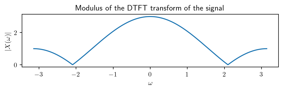
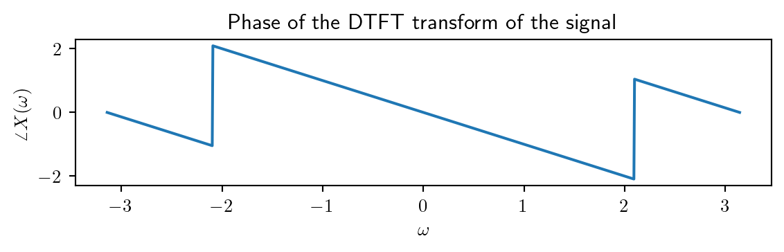
|X(\omega)| &= \sqrt{(1 + \cos(\omega) + \cos(2\omega))^2 + (\sin(\omega) + \sin(2\omega))^2} \\
\angle{X(\omega)} &= \arctan\left(\frac{- \sin(\omega) - \sin(2\omega)}{1 + \cos(\omega) + \cos(2\omega)}\right)
\end{aligned}\]
Just for fun, we can plot these functions here:
Code
import numpy as npimport matplotlib.pyplot as plt#%matplotlib inlineplt.rcParams['text.usetex'] =Truew = np.linspace(-np.pi, np.pi, 1000)X =1+ np.cos(w) + np.cos(2*w) -1j*(np.sin(w) + np.sin(2*w))plt.figure(figsize=(6, 2))plt.plot(w, np.abs(X))plt.xlabel(r'$\omega$')plt.ylabel(r'$|X(\omega)|$')plt.title('Modulus of the DTFT transform of the signal')plt.tight_layout()plt.figure(figsize=(6, 2))plt.plot(w, np.angle(X))plt.xlabel(r'$\omega$')plt.ylabel(r'$\angle{X(\omega)}$')plt.title('Phase of the DTFT transform of the signal')plt.tight_layout()
b). What is the signal’s spectrum (modulus and phase) at frequency \(f=\frac{1}{2}\)?
We have to evaluate the expressions for \(|X(\omega)|\) and \(\angle{X(\omega)}\) at \(\omega = 2\pi f = 2 \pi \frac{1}{2} = \pi\):
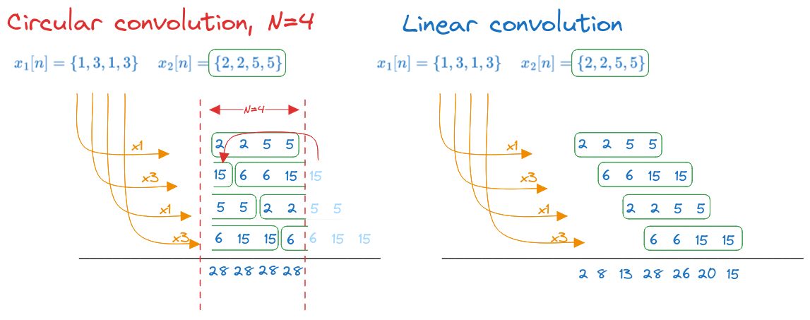
Compute the circular convolution of the two signals: \[x_1[n] = [1, 3, 1, 3]\]\[x_2[n] = [2, 2, 5, 5]\]
Solution
We can use the definition of the circular convolution: \[y[n] = x_1[n] \circledast x_2[n] = \sum_{m=0}^{N-1} x_1[m] x_2[(n-m) \mod N]\]
where \(N\) is the length of the signals. In this case, \(N=4\).
We follow the same procedure as when calculating the linear convolution, but the indices (positions) are wrapped by \(N\). When we exceed the length of the signal, we shift the position back to the beginning.
Circular convolution vs linear convolution
The result is a sequence with the same length as the input sequences, \(N=4\): \[y[n] = x_1[n] \circledast x_2[n] = [28, 28, 28, 28]\]
WarningCoincidence
It is only a coincidence that all the values of \(y[n]\) are equal here, \([28, 28, 28, 28]\). In general, the result could be anything.
TipGeneralizations
If the two signals have different lengths, we append zeros to the shorter one until both have the same length.
We can pick any value if \(N\) longer than the signals. In this case, we extend both signals with zeros until the prescribed length. This is called the circular convolution in N points.
Homework: compute the circular convolution of these signals in \(N=6\) points.
If \(N\) is large enough, the circular convolution becomes the linear convolution. \(N\) must be larger than \(Length_1 + Length_2 - 1\).
Homework: compute the circular convolution of these signals in \(N=7\) points.
7.3 Exercise 3
Compute the circular convolution in \(N = 7\) points of the same two signals
Solution
We must append zeros to both signals to make their length 7, then do circular convolution as before.
Surprise: we obtain the same result as linear convolution.
7.4 Exercise 4
Consider a periodic signal \(x[n]\) with period \(N=6\) and the DFT coefficients:
It is not a coincidence that \(X_4 = X_2^*\) and \(X_5 = X_1^*\). If the signal \(x[n]\) has real values, then there is always this complex conjugate property, because the DFT coefficients are even: \[X_k = X_{k-N} = X_{N-k}^*\]
7.5 Exercise 5
Consider a periodic signal \(x[n]\) with period \(N=5\) and the DFT coefficients:
Note that \(X_3 = X_{3-N} = X_{-1} = X_1^*\), as expected.
Second, we write the signal as a sum of sinusoidal components, using the formula for \(N\) even from the previous exercises: \[x[n] = \frac{1}{N} X_0 + \frac{1}{N} \sum_{k=1}^{N/2-1} 2 |X_k| \cos\left( 2\pi \frac{k}{N} n + \angle{X_k}\right) + \frac{1}{N} |X_{N/2}| \cos\left( \pi n + \angle{X_{N/2}}\right)\]
The modulus and phase of the DFT coefficients are:
Therefore we can write the signal as: \[\begin{aligned}
x[n] &= \frac{1}{4} \cdot 2 + \frac{1}{4} \cdot 2 \sqrt{2} \cos\left( 2\pi \frac{1}{4} n - \frac{\pi}{4}\right)\\
&= \frac{1}{2} + \frac{\sqrt{2}}{2} \cos\left( \frac{\pi}{2} n - \frac{\pi}{4}\right)
\end{aligned}\]
The constant DC component is \(\frac{1}{2}\), and there is one sinusoidal component with frequency \(f=\frac{1}{4}\), amplitude \(\frac{\sqrt{2}}{2}\) and initial phase \(-\frac{\pi}{4}\).
7.7 Exercise 7
Write the DFT calculation in Ex.5 as a matrix multiplication.
Solution
This is just a straightforward illustration of the theory.
Note that we can write the calculations for \(X_k\) as the following matrix-vector multiplication: \[\begin{bmatrix}
X_0 \\
X_1 \\
X_2 \\
X_3
\end{bmatrix} = \begin{bmatrix}
1 & 1 & 1 & 1 \\
1 & e^{-j \pi/2} & e^{-j 2\pi/2} & e^{-j 3\pi/2} \\
1 & e^{-j \pi} & e^{-j 2\pi} & e^{-j 3\pi} \\
1 & e^{-j 3\pi/2} & e^{-j 6\pi/2} & e^{-j 9\pi/2}
\end{bmatrix} \begin{bmatrix}
x[0] \\
x[1] \\
x[2] \\
x[3]
\end{bmatrix}\]
Welcome to the world of linear algebra and orthogonal transformations!
7.8 Exercise 8
Compute \(x[n]\) in Ex.4 and Ex.5, in two ways:
using the definition formula
using the matrix form
Solution
We have to compute the signal \(x[n]\) from the DFT coefficients \(X_k\) that are provided in the exercises.
We can achieve this in many ways:
Since we have \(x[n]\) written as a sum of sinusoids, we can just give values to \(n=0, 1, 2, 3, 4, 5\) and compute the values.
We can use the definition formula of the Inverse DFT, IDFT: \[x[n] = \frac{1}{N} \sum_{k=0}^{N-1} X_k e^{j 2\pi \frac{k}{N} n}\]
We can use the matrix form, which uses the transposed and conjugated matrix of the one used in the DFT calculation:
7.8.0.1 Variant 1: using the sum of sinusoids
We have already written \(x[n]\) as a sum of sinusoids in the previous exercises.
We have to evaluate those expressions for \(n=0, 1, 2, 3, ... , N-1\).
7.8.0.2 Variant 2: using the IDFT formula
The Inverse DFT (IDFT) formula is: \[x[n] = \frac{1}{N} \sum_{k=0}^{N-1} X_k e^{j 2\pi \frac{k}{N} n}, n=0,1,...,N-1\] We have to compute \(N\) sums, each with \(N\) terms.
The matrix is fixed (depends only on \(N=6\), not on the signal), so the multiplication is straightforward.
We won’t actually compute this, by hand. We could use MATLAB or Python to do it. Note that there is an even faster way to compute this, using the Fast Fourier Transform (FFT) algorithm.
A signal \(x[n]\) has a Z transform with one pole \(p_1 = -0.5\) and one zero \(z_1 = 0.9\). It is known that at \(\omega = \pi\), the modulus of the Fourier transform is \(|X(\omega=\pi)| = 1\).
Find the signal’s Z transform \(X(z)\)
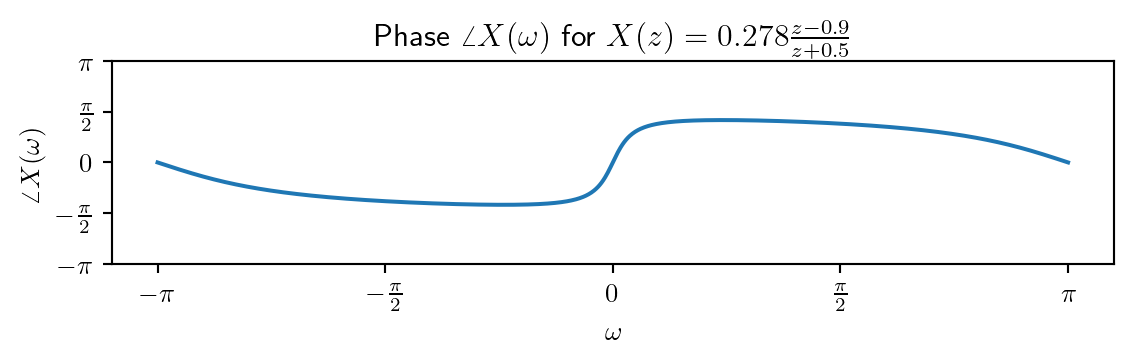
Compute the expression of \(|X(\omega)|\) and \(\angle X(\omega)\)
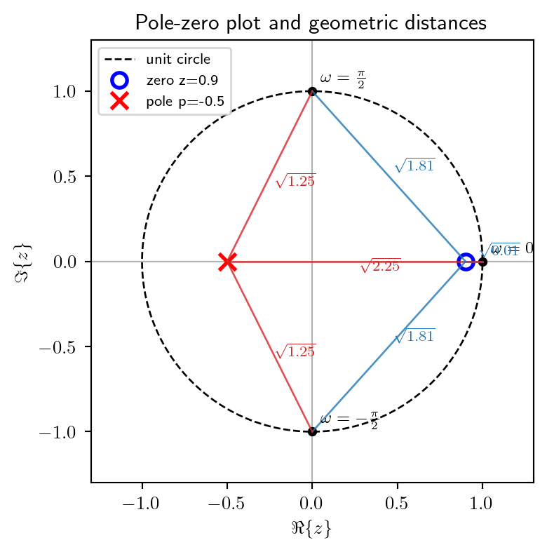
Find the values \(|X(\frac{\pi}{2})|\), \(|X(\frac{-\pi}{2})|\) and \(|X(0)|\)
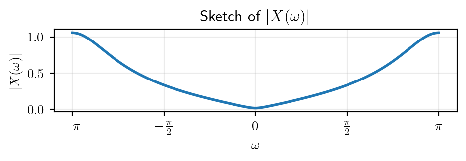
Sketch \(|X(\omega)|\)
Solution
a). Find the signal’s Z transform \(X(z)\)
Since there is one zero \(z_1 = 0.9\), the Z transform has one term \((z - 0.9)\) at the numerator.
Since there is one pole \(p_1 = -0.5\), there is a term \((p + 0.5)\) at the denominator.
Therefore, the Z transform looks like this:
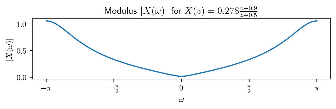
\[X(z) = G \frac{z-0.9}{z + 0.5}\]
There is still a scaling factor \(G\) (“gain”) in front which we have to find. The poles and zeros do not tell us anything about the value of the gain factor. This can be found from the additional information that \(|X(\omega=\pi)| = 1\) (in general, from the value of \(X(z)\) or \(X(\omega)\) in one given point).
Indeed, we turn \(X(z)\) into \(X(\omega)\) replacing \(z = e^{j\omega}\):
\[X(\omega) = G \frac{e^{j \omega}-0.9}{e^{j \omega} + 0.5}\]
and for \(\omega = \pi\) we have \(e^{j\pi} = -1\), which means:
These two expressions may look complicated, and indeed they are, but they are useful. For example, we can now plot them, and take a look at the Fourier transform:
a). low frequency content b). frequency content around the frequency \(\omega = \frac{\pi}{2}\)
Solution
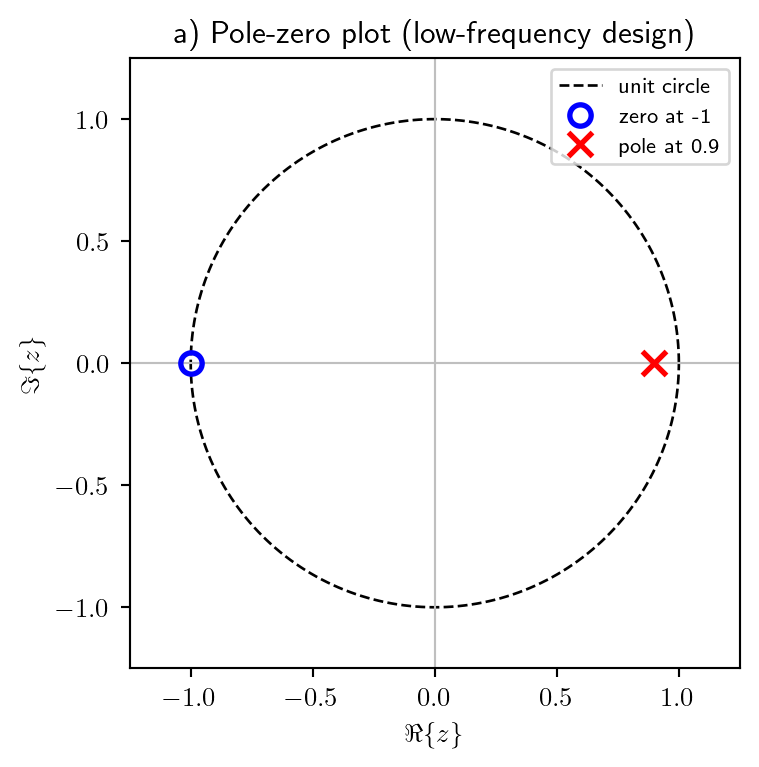
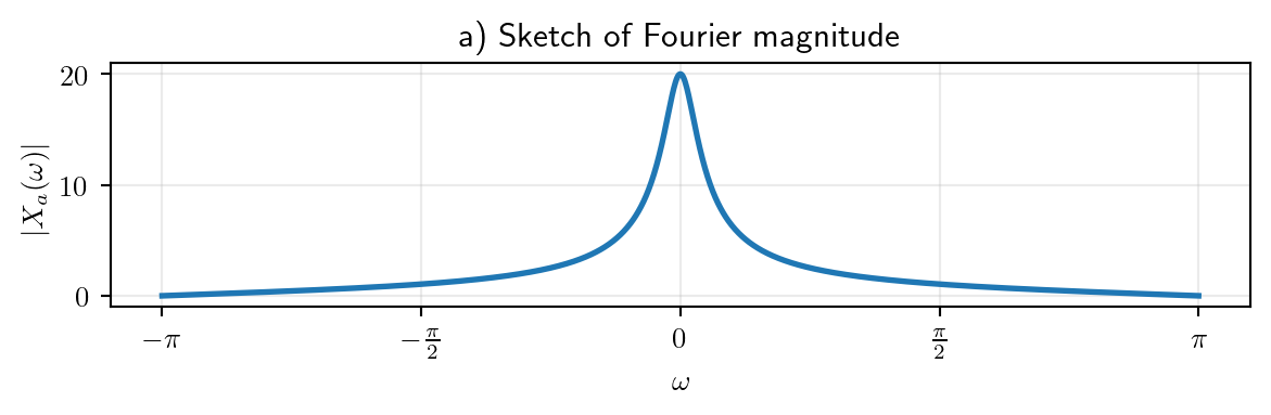
a). Signal with low-frequency content
We consider the following pole-zero plot. The pole is close to the point \(1\), but not quite on the unit circle (for stability reasons), e.g. \(p = 0.9\). The zero is precisely on the unit circle, at point \(-1\).
Code
pa = [0.9] # one pole near z=1za = [-1] # one zero at z=-1fig, ax = plt.subplots(figsize=(4.3, 4.1))t = np.linspace(0, 2*np.pi, 500)ax.plot(np.cos(t), np.sin(t), 'k--', lw=1, label='unit circle')ax.axhline(0, color='0.75', lw=0.8)ax.axvline(0, color='0.75', lw=0.8)ax.plot(np.real(za), np.imag(za), 'ob', ms=8, mfc='none', mew=2, label='zero at -1')ax.plot(np.real(pa), np.imag(pa), 'xr', ms=9, mew=2, label='pole at 0.9')ax.set_aspect('equal', adjustable='box')ax.set_xlim(-1.25, 1.25)ax.set_ylim(-1.25, 1.25)ax.set_xlabel(r'$\Re\{z\}$')ax.set_ylabel(r'$\Im\{z\}$')ax.set_title(r'a) Pole-zero plot (low-frequency design)')ax.legend(loc='upper right', fontsize=8)plt.tight_layout()
Interpretation of the pole-zero plot using the geometrical method:
near \(\omega \approx 0\), the point \(e^{j\omega}\) is close to the pole at \(0.9\), so denominator distance is small and \(|X_a(\omega)|\) is large
near \(\omega \approx \pi\), the point \(e^{j\omega}\) is close to the zero at \(-1\), so numerator distance is small and \(|X_a(\omega)|\) is small
exactly at \(\omega = \pi\), the point \(e^{j\omega}\) is exactly in the zero at \(-1\), so numerator is \(0\) and \(|X_a(\omega)| = 0\)
So the Fourier transform is dominated by low frequencies.
The sketch of the Fourier transform magnitude obtained in this way shows it is low frequency:
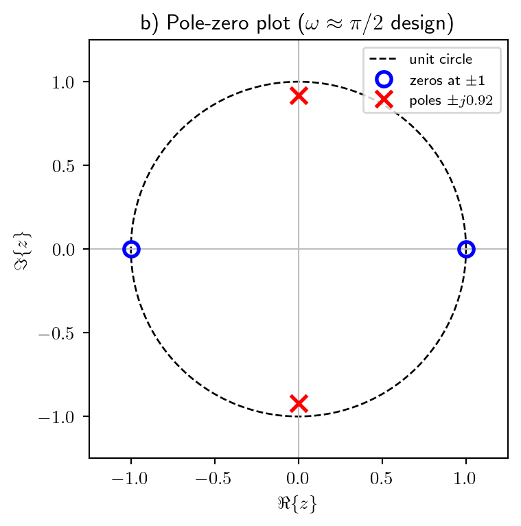
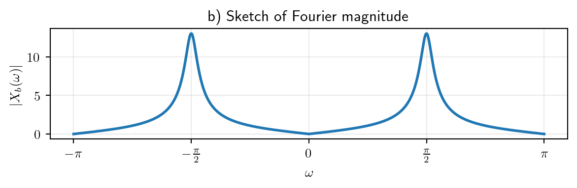
b). Signal with frequency content around \(\omega = \frac{\pi}{2}\)
We consider the following pole-zero plot. The poles are selected close to the unit circle, but not quite on it (for stability), e.g. \(p_{1,2} = \pm j 0.95\). The zeros are precisely in the values \(1\) and \(-1\).
Code
r =0.92pb = [1j*r, -1j*r] # conjugate pole pair near omega = +/- pi/2zb = [1, -1] # two zeros at z=1 and z=-1fig, ax = plt.subplots(figsize=(4.3, 4.1))t = np.linspace(0, 2*np.pi, 500)ax.plot(np.cos(t), np.sin(t), 'k--', lw=1, label='unit circle')ax.axhline(0, color='0.75', lw=0.8)ax.axvline(0, color='0.75', lw=0.8)ax.plot(np.real(zb), np.imag(zb), 'ob', ms=8, mfc='none', mew=2, label='zeros at ±1')ax.plot(np.real(pb), np.imag(pb), 'xr', ms=9, mew=2, label=r'poles $\pm j0.92$')ax.set_aspect('equal', adjustable='box')ax.set_xlim(-1.25, 1.25)ax.set_ylim(-1.25, 1.25)ax.set_xlabel(r'$\Re\{z\}$')ax.set_ylabel(r'$\Im\{z\}$')ax.set_title(r'b) Pole-zero plot ($\omega\approx\pi/2$ design)')ax.legend(loc='upper right', fontsize=8)plt.tight_layout()
Interpretation of the pole-zero plot using the geometrical method:
near \(\omega \approx \frac{\pi}{2}\) and \(-\frac{\pi}{2}\), \(e^{j\omega}\) is close to poles, so denominator distances are small and \(|X_b(\omega)|\) is large
near \(\omega \approx 0\) and \(\omega \approx \pi\), \(e^{j\omega}\) is close to zeros at \(1\) and \(-1\), so numerator distances are small and \(|X_b(\omega)|\) is small
precisely at \(\omega = 0\) and \(\omega = \pi\), \(e^{j\omega}\) is exactly in the zeros at \(1\) and \(-1\), so numerator distances are zero and \(|X_b(\omega)| = 0\)
So the Fourier transform has strong content around \(\omega=\pm\frac{\pi}{2}\) and attenuation around \(\omega=0,\pi\).