This function \(e^{jx}\) is known as the complex exponential.
relation between \(\cos()\) and \(\sin()\) and the complex exponential: \[
\begin{split}
\cos(x) &= \frac{e^{jx} + e^{-jx}}{2}\\
\sin(x) &= \frac{e^{jx} - e^{-jx}}{2j}\\
\end{split}
\]
\(\cos()\) and \(\sin()\) are just shifted versions of each other: \[
\begin{split}
\sin(x) &= \cos(x - \frac{\pi}{2})\\
\cos(x) &= \sin(x + \frac{\pi}{2})
\end{split}
\]
2.2.1 Eigen-signals of LTI systems
Why are sinusoidal signals \(\sin()\) and \(\cos()\) so prevalent in signal processing? The reason is that they can be written based on \(e^{jx}\) and an \(e^{-jx}\). In fact, it is the function \(e^{jx}\) that is very special, due to its relation to differential equations, and \(\sin()\) and \(\cos()\) merely inherit the nice properties of \(e^{jx}\).
Why is the function \(e^{jx}\) special? From the point of view of LTI systems, it is because it is an eigen-function of these systems.
An eigen-function (“funcție proprie”) of a mathematical system is function \(f\) which, if input in a system, produces an output proportional to it: \[H\lbrace f \rbrace = \lambda \cdot f, \lambda \in \mathbb{C}\]
Using the signal processing terminology, a signal \(x[n]\) is called an eigen-signal of the system if the output signal is proportional to the input signal: \[y[n] = H \lbrace x[n] \} = \lambda \cdot x[n]\] It turns out that the complex exponential signals \(e^{j\omega n}\) are eigen-signals of Linear and Time Invariant (LTI) systems.
NoteTheorem: Complex exponentials are eigen-signals of LTI systems
The complex exponential signals \(e^{j\omega n}\) are eigen-functions of Linear and Time Invariant (LTI) systems: \[
y[n] = H \lbrace x[n] \} = \lambda \cdot x[n], \lambda \in \mathbb{C}, \forall H{} \textrm{ a LTI system}
\]
Proof: Let’s consider an input signal \(x[n] = A e^{j\omega_0 n}\), for some values \(A\), \(\omega_0 \in \mathbb{R}\).
The LTI system \(H\) has an impulse response \(h[n]\). The output signal is the convolution of the input signal \(x[n]\) with the impulse response \(h[n]\): \[
\begin{split}
y[n] &= \sum_{k=-\infty}^\infty h[k] x[n-k]\\
&= \sum_{k=-\infty}^\infty h[k] A e^{j \omega_0 (n-k)} \\
&= \sum_{k=-\infty}^\infty h[k] e^{-j \omega_0 k} A e^{j \omega_0 n}\\
&= A e^{j \omega_0 n} \underbrace{\sum_{k=-\infty}^\infty h[k] e^{-j \omega_0 k}}_{H(\omega_0)}\\
&= H(\omega_0) \cdot x[n]
\end{split}
\]
With the notation \(H(\omega_0) = \sum_{k=-\infty}^\infty h[k] e^{-j \omega_0 k}\), which is a constant complex number, we have shown that \(y[n]\) is proportional to \(x[n]\): \[
y[n] = H(\omega_0) \cdot x[n]
\]
The concept of eigen-signals and, more generally, of eigen-functions, is similar to the concept of eigen-vectors of a matrix (remember algebra). Eigen-vectors are vectors which, when multiplied by a matrix \(A\), produce a vector proportional to the input vector. \[
A \cdot v = \lambda \cdot v
\] The core idea is the same: the vector \(v\) is not changed by the matrix \(A\) except by scaling with some value.
Eigen-signals are very useful as building blocks of signals. If we can decompose a signal into a sum of eigen-signals, we can easily understand how the signal will be transformed by LTI a system, since each of the eigen-signals will be transformed into a scaled version of itself. The output signal will be a sum of scaled versions of the input signal’s eigen-signals.
This is exactly the idea behind the Fourier Transform. The Fourier Transform decomposes a signal into a sum of complex exponentials \(e^{j\omega n}\), so that when the signal passes through an LTI system, we can understand the effect as simply scaling each of the complex exponentials (multiplication by the transfer function \(H(\omega)\)).
TipExample
2.2.1.1 Example
Imagine a professional DSLR photo camera with some RGB color filters mounted on the lens. Suppose we have three photographic filters which reduce the intensity of the red, green, and blue colors:
one filter reduces red to 50%: \[R_{out} = 0.5 \cdot R_{in}\]
one filter reduces green to 25%: \[G_{out} = 0.25 \cdot G_{in}\]
one filter reduces blue to 80%: \[B_{out} = 0.8 \cdot B_{in}\]
The colors R, G, B behave like eigen-colors of the system, in the sense that the output is proportional to the input.
Now, suppose we have an input color “pink” which is some combination of red and blue. What is the output color if we pass the “pink” color through the filters?
The answer is easy if we represent the “pink” color in terms of the eigen-colors R, G, B. If, say, pink is equal to \(200 \cdot R + 0 \cdot G + 200 \cdot B\), then the output will simply be: \[
200 \cdot 0.5 \cdot R + 0 \cdot 0.25 \cdot G + 200 \cdot 0.8 \cdot B
\]
Decomposing the color in terms of the eigen-colors R, G, B, makes it easy to understand the effect of the filters. R, G, B are the natural way of representing colors in this case, making it easy to understand the effect of the filters.
2.2.2 The Fourier Transforms
The Fourier Transform is the mathematical tool that allows us to decompose a signal as a linear combination of complex exponentials \(e^{j\omega n}\).
For non-periodic signals, we use the Discrete-Time Fourier Transform (DTFT) and its inverse.
A signal \(x[n]\) can be written as an infinite sum (i.e. integral) of complex exponentials: \[x[n] = \int_{f=-1/2}^{1/2} X(f) e^{j 2 \pi f n} df\] with some coefficients, \(X(f)\).
Discrete-Time Fourier Transform (DTFT):
The coefficients \(X(f)\) are found as: \[X(f) = \langle x[n], e^{j 2 \pi f n} \rangle = \sum_{n=-\infty}^{\infty} x[n] e^{- j 2 \pi f n}\]
Alternatively, we can write these in terms of \(\omega\), by replacing \(f\) with \(\omega = 2 \pi f\) and \(df = \frac{1}{2 \pi} d\omega\): \[
\begin{split}
x[n] &= \frac{1}{2 \pi}\int_{\omega=-\pi}^{\pi} X(\omega) e^{j \omega n} d\omega\\
X(\omega) &= \langle x[n], e^{j \omega n} \rangle = \sum_n x[n] e^{- j \omega n}
\end{split}
\]
For periodic signals, we use the Discrete Fourier Transform (DFT) formula and its inverse, because the spectrum \(X(f)\) is discrete, so there is just a finite number of coefficients:
Inverse Discrete Fourier Transform (Inverse DFT):
A periodic signal \(x[n]\) can be written as a sum of exactly \(N\) complex exponentials: \[ x[n] = \frac{1}{N} \sum_{k=0}^{N-1} X_k e^{j 2 \pi k n / N} \] with some coefficients, \(X_k\).
Discrete Fourier Transform (DFT):
The coefficients \(X_k\) are found as: \[X_k = \langle x[n], e^{j 2 \pi f n} \rangle = \sum_{n=0}^{N-1} x[n] e^{- j 2 \pi k n / N}\]
In the following, we shall analyze each variant of the Fourier Transform in more detail.
2.3 The Discrete-Time Fourier Transform (DTFT)
The Discrete-Time Fourier Transform (DTFT) is used for discrete signals, infinitely long, that are non-periodic.
The inverse DTFT shows that a signal can be written as a continuous sum (i.e. an intergal) of complex exponentials \(e^{j \omega n}\), with some coefficients \(X(\omega)\) or \(X(f)\). The direct DTFT shows how to compute these coefficients.
2.3.1 Basic properties of DTFT
The function \(X(\omega)\) is known as the spectrum of the signal \(x[n]\).
\(X(\omega)\) is defined only for \(\omega \in [-\pi, \pi]\), or \(f \in [-\frac{1}{2}, \frac{1}{2}]\). This is unlike the spectrum of continuous signals, which ranges from \(-\infty\) to \(\infty\).
\(X(\omega)\) is has complex values, meaning there exists the functions \(| X(\omega) |\) and \(\angle X(\omega)\).
If the signal \(x[n]\) is real, \(X(\omega)\) is even: \[x[n] \in \mathbb{R} \rightarrow X(-\omega) = X^*(\omega)\]
Furthermore, this means that the modulus \(|X(\omega)|\) is an even, real-valued function: \[|X(\omega)| = |X(-\omega)|\] and the phase \(\angle X(\omega)\) is an odd, real-valued function: \[X(\omega) = - X(-\omega)\]
2.3.2 Sum of sinusoids
The Inverse DTFT can be rewritten to show the signal \(x[n]\) as a sum of sinusoids.
By grouping terms with \(e^{j \omega n}\) and \(e^{j (-\omega) n}\) we get:
The Inverse DTFT shows, therefore, that any signal \(x[n]\) can be written as a continuous sum (i.e. integral) of sinusoids with all frequencies \(f \in [-\frac{1}{2}, \frac{1}{2}]\).
The coefficient of each sinusoid is given by the spectrum \(X(f)\), for every value of \(f\):
The modulus\(|X(\omega)|\) gives the amplitude of the sinusoids (\(\times\) 2)
As a particular case for \(\omega = 0\), \(|X(\omega=0)|\) gives the DC component of the signal
The phase\(\angle X(\omega)\) gives the initial phase shift of the sinusoids
This is the fundamental practical interpretation of the Fourier transform: it shows that any signal can be decomposed into a continuous sum of sinusoids of all frequencies, each with a certain amplitude and phase.
2.3.3 Properties of DTFT
2.3.3.1 Linearity
The DTFT is a linear operation. The DTFT of a linear combination of signals is the linear combination of their DTFTs: \[a \cdot x_1[n] + b\cdot x_2[n] \leftrightarrow a \cdot X_1(\omega)+ b\cdot X_2(\omega)\]
Proof: via definition
2.3.3.2 Shifting in time
The DTF of a signal delayed by \(n_0\) is the DTFT of the original signal, multiplied by a complex exponential:
Note that \[ | e^{-j \omega n_0} X(\omega) | = | X(\omega) |\] which shows that when a signal is shifted in time, the amplitudes \(|X(\omega)|\) of the spectrum are not affected. Shifting in time affects only the phase of the spectrum. This makes sense, because shifting a signal in time does not change the “amplitudes” of the composing sinusoids, it only shifts them.
2.3.3.3 Modulation in time
A shift of the spectrum \(X(\omega)\) by \(\omega_0\) corresponds to a modulation of the signal \(x[n]\) by a complex exponential:
The cross-correlation of two signals in time domain corresponds to the product of their spectra in frequency domain, the second spectrum being complex conjugated:
Note that this is a special case of the correlation theorem, where the two signals are the same: \[r_{xx}[l] \leftrightarrow X(\omega) X^*(\omega) = |X(\omega)|^2\] since for any complex number \(z\), \(z \cdot z^* = |z|^2\).
2.3.3.9 Parseval theorem
The Parseval theorem states that the energy of the signal is the same in time and frequency domains: \[E = \sum_{-\infty}^\infty |x[n]|^2 = \frac{1}{2 \pi}\int_{-\pi}^\pi |X(\omega)|^2\]
The energy of a function, in general, is defined as the sum of the squares of its values. In the case of a signal, in the time domain we have the sum of the squares of the samples, and in the frequency domain we have the integral of the square of the spectrum, since the spectrum is continuous.
2.3.4 Relation between DTFT and Z transform
The DTFT is a special case of the Z transform, where the Z transform is evaluated on the unit circle, i.e. with \[z = e^{j \omega}\]
This is clearly seen from the definitions of the DTFT and Z transforms, where replacing \(z = e^{j \omega}\) in the Z transform leads to the DTFT:
Z transform: \[X(z) = \sum_n x[n] z^{-n}\]
DTFT: \[X(\omega) = \sum_n x[n] e^{-j \omega n}\]
The points defined by \(z = e^{j \omega}\) are points on the unit circle, since the modulus of such \(z\) is 1: \[|z| = |e^{j \omega}| = 1\] The phase (angle) of these points \(z\) is \(\omega\): \[\angle{z} = \angle{e^{j \omega}} = \omega\]
We say therefore that the DTFT is the Z transform evaluated on the unit circle. This requires that the Z transform converges on the unit circle, which is the case for most usual signals. Otherwise, the equivalence does not hold
2.4 The Discrete Fourier Transform (DFT)
The Discrete Fourier Transform (DFT) is used for discrete signals, periodic, with period \(N\).
If we apply the DTFT to a periodic signal, we get a spectrum that is discrete, with only \(N\) Dirac deltas. In this case it is easier to replace the integral with a sum of exactly \(N\) terms, and in this way we get the DFT.
Inverse Discrete Fourier Transform (Inverse DFT) \[x[n] = \frac{1}{N} \sum_{k=0}^{N-1} X_k e^{j 2 \pi k n / N}\]
Discrete Fourier Transform (DFT): \[X_k = \langle x[n], e^{j 2 \pi f n} \rangle = \sum_{n=0}^{N-1} x[n] e^{- j 2 \pi k n / N}\]
The DFT is defined for periodical signals with period \(N\), and there are exactly \(N\) terms in each sum in the two formulas above. The DFT formula only uses the values from one period of the signal, \(x[n]\) for \(n = 0, 1, \dots, N-1\), because the signal is periodic and the values repeat from \(N\) onwards.
NoteNote
Remember the differences between the DTFT and DFT in terms of the types of signals and spectra:
The DFT takes a vector with N elements (\(x[0], \dots, x[N-1]\)) and produces a vector with N elements (\(X_k\)). For this reason, we can compute it with tools like Matlab, because it is a finite operation.
The DTFT takes an infinitely-long signal \(x[n]\) and produces a continuous function (\(X(\omega)\)) between \([-\pi, \pi]\).
2.4.1 Basic properties of DFT
The DFT produces only \(N\) coefficients \(X_k\), with each \(X_k\) corresponding to a frequency \(f = \frac{k}{N}\). \(X_0\) corresponds to the DC component, \(X_1\) to the frequency \(f = \frac{1}{N}\), and so on.
The DFT coefficients \(X_k\) are complex numbers, meaning they have a modulus \(|X_k|\) and a phase \(\angle X_k\).
If the signal \(x[n] \in \mathbb{R}\), the coefficients are even (and complex): \[X_{-k} = X_k^*\] Furthermore, this means that the modulus \(|X_k|\) are even, real values: \[|X_{-k}| = |X_k|\] and the phase \(\angle X_k\) are odd, real values: \[\angle X_{-k} = -\angle X_k\]
The DFT coefficients \(X_k\) are periodic with period \(N\), i.e. \(X_{k+N} = X_k\). This can be shown from the DFT formula, where, if we replace \(k\) with \(k + N\), we get the same value: \[
\begin{split}
X_{k+N} &= \sum_{n=0}^{N-1} x[n] e^{- j 2 \pi (k + N) n / N}\\
&= \sum_{n=0}^{N-1} x[n] e^{- j 2 \pi k n / N} e^{- j 2 \pi n}\\
&= \sum_{n=0}^{N-1} x[n] e^{- j 2 \pi k n / N}\\
&= X_k
\end{split}
\] The periodicity of the DFT coefficients is the reason for which the Inverse DFT only uses the values \(X_0, X_1, \dots, X_{N-1}\), since the values repeat afterwards.
Because of periodicity, we can rename the coefficients \(X_{N-k}\) as \(X_{-k}\). Consider, for example, a signal \(x[n]\) with period \(N = 6\). The signal has 6 DFT coefficients \(X_0\), \(X_1\), \(X_2\), \(X_3\), \(X_4\), \(X_5\). However, we can rename the last ones as \(X_5 = X_{-1}\), and \(X_4 = X_{-2}\). Thus, the 6 coefficients can be considered \(X_{-2}\), \(X_{-1}\), \(X_0\), \(X_1\), \(X_2\), \(X_3\).
This “renaming” of coefficients corresponds to the fact that the frequency \(f = \frac{N-k}{N}\) is the same as \(f - 1 = \frac{-k}{N}\), which we know from the aliasing effect. Thus, for a periodic signal with \(N=6\), the coefficient \(X_5\) corresponds to frequency \(f = \frac{5}{6}\), which is the same as \(f = \frac{-1}{6}\), which corresponds to \(X_{-1}\). Similarly, \(X_4\) corresponds to \(f = \frac{4}{6}\), which is the same as \(f = \frac{-2}{6}\), which corresponds to \(X_{-2}\). The resulting DFT coefficients are \(X_{-2}\), \(X_{-1}\), \(X_0\), \(X_1\), \(X_2\), \(X_3\), and now their corresponding frequencies are all in the range \([-\frac{1}{2}, \frac{1}{2}]\).
2.4.2 Sum of sinusoids
Just like the DTFT, the DFT can be rewritten to show the signal \(x[n]\) as a sum of sinusoids, where the modulus \(|X_k|\) gives the amplitude of the sinusoids, and the phase \(\angle X_k\) gives the initial phase shift.
For easy analysis, we consider seperately the cases when \(N\) is odd and when \(N\) is even.
2.4.2.1 Sum of sinusoids with N = odd
If \(N\) is odd, we have an odd number of coefficients \(X_k\). We keep \(X_0\) single, and we group together the coefficients \(X_k\) and \(X_{-k}\) as follows:
\[\begin{split}
x[n] &= \sum_{k=-(N-1)/2}^{(N-1)/2} X_k e^{j 2 \pi k n / N}\\
&= \frac{1}{N} X_0 e^{j 0 n} + \frac{1}{N} \sum_{k=-(N-1)/2}^{-1} X_k e^{j 2 \pi k n / N} + \frac{1}{N} \sum_{k=1}^{(N-1)/2} X_k e^{j 2 \pi k n / N}\\
&= \frac{1}{N} X_0 + \frac{1}{N} \sum_{k=1}^{(N-1)/2} (X_k e^{j 2 \pi k n / N} + X_{-k} e^{- j 2 \pi k n / N} )\\
&= \frac{1}{N} X_0 + \frac{1}{N} \sum_{k=1}^{(N-1)/2} |X_k| ( e^{j 2 \pi k n /N + \angle{X(k)}} + e^{- j 2 \pi k n / N - \angle{X(\omega)}} )\\
&= \frac{1}{N} X_0 + \frac{1}{N} \sum_{k=0}^{(N-1)/2} 2 |X_k| \cos(2 \pi k/N n + \angle X_k)
\end{split}\]
This shows that a signal \(x[n]\) with period \(N\) can be written as a sum of a few sinusoids with frequencies \(0, \frac{1}{N}, \frac{2}{N}, \dots\), not exceeding 1/2.
The DC component is given by \(X_0\). The amplitudes of the sinusoids are given by \(|X_k|\), and the phases by \(\angle X_k\).
2.4.2.2 Sum of sinusoids with N = even
If \(N\) is even, we have an even number of coefficients \(X_k\). We group together the coefficients \(X_k\) and \(X_{-k}\) as follows: - we leave \(X_0\) on its own - we group \(X_1\) and \(X_{-1}\), \(X_2\) and \(X_{-2}\), and so on - there is one remaining coefficient \(X_{N/2}\), which has no pair
For example, for \(N=6\), we have coefficients \(X_{-2}, X_{-1}, X_0, X_1, X_2, X_3\). We group \(X_1\) and \(X_{-1}\), \(X_2\) and \(X_{-2}\), while \(X_0\) and \(X_3\) are left on their own.
We observe that the final term \(X_{N/2}\), having no pair, must be a real number. Because of periodicity, we must have $X_{N/2} = X_{-N/2}, but on other hand toe coefficients are even, so \(X_{N/2} = X_{-N/2}^*\). This means that \(X_{N/2}\) is equal to its own complex conjugate, so it must be a real number.
We have:
\[\begin{split}
x[n] &= \sum_{k=-(N-2)/2}^{N/2} X_k e^{j 2 \pi k n / N}\\
&= \frac{1}{N} X_0 e^{j 0 n} + \frac{1}{N} \sum_{k=-(N-2)/2 }^{-1} X_k e^{j 2 \pi k n / N} + \frac{1}{N} \sum_{k=1}^{(N-2)/2} X_k e^{j 2 \pi k n / N} + \frac{1}{N} X_{N/2} e^{j 2 \pi (N/2) n / N}\\
&= \frac{1}{N} X_0 + \frac{1}{N} \sum_{k=1}^{(N-2)/2} (X_k e^{j 2 \pi k n / N} + X_{-k} e^{- j 2 \pi k n / N} ) + \frac{1}{N} X_{N/2} e^{j 2 \pi (N/2) n / N}\\
&= \frac{1}{N} X_0 + \frac{1}{N} \sum_{k=1}^{(N-2)/2} 2 |X_k| \cos(2 \pi k/N n + \angle X_k) + \frac{1}{N} X_{N/2} \cos(n \pi)
\end{split}\]
This shows that a signal \(x[n]\) with period \(N\) can be written as a sum of a few sinusoids with frequencies \(0, \frac{1}{N}, \frac{2}{N}, \dots\), up to but not exceeding 1/2.
The DC component is given by \(X_0\).
The amplitudes of the sinusoids are given by \(|X_k|\), and the phases by \(\angle X_k\). Note that for the frequency \(1/2\) in particular, (the last term in the sum), the amplitude is \(X_{N/2}\), which is a real number, and doesn’t have the factor of 2. Also, its phase is 0, because \(X_{N/2}\) is real.
TipExercises
Consider a periodic signal \(x[n]\) with period \(N=6\) and the DFT coefficients:
A particularly useful way to think about the DFT is as a matrix multiplication. Indeed, applying the DFT to a signal \(x[n]\) of length N (i.e. one period) is equivalent to multiplying the signal by a matrix \(\mathbf{W}_N\) of size \(N \times N\): \[\mathbf{X} = \mathbf{W}_N \cdot \mathbf{x}\] i.e.: \[
\begin{bmatrix}
X_0 \\
X_1 \\
\vdots \\
X_{N-1}
\end{bmatrix}
=
\underbrace{
\frac{1}{\sqrt{N}} \begin{bmatrix}
1 & 1 & 1 & \cdots & 1 \\
1 & w & w^2 & \cdots & w^{N-1} \\
1 & w^2 & w^4 & \cdots & w^{2(N-1)} \\
\vdots & \vdots & \vdots & \ddots & \vdots \\
1 & w^{N-1} & w^{2(N-1)} & \cdots & w^{(N-1)(N-1)}
\end{bmatrix}
}_{\mathbf{W}_N}
\cdot
\begin{bmatrix}
x[0] \\
x[1] \\
\vdots \\
x[n-1]
\end{bmatrix}
\] where \(w = e^{-j \frac{2\pi}{N}}\) is the \(N\)-th root of unity.
The inverse DFT is also a matrix multiplication, with the inverse matrix \(\mathbf{W}_N^{-1}\) which is the conjugate transpose of \(\mathbf{W}_N\): \[\mathbf{x} = \mathbf{W}_N^{-1} \cdot \mathbf{X}\] with: \[\mathbf{W}_N^{-1} = \mathbf{W}_N^T\]
The DFT matrix \(\mathbf{W}_N\) is a unitary matrix, meaning that its inverse is its conjugate transpose.
There might be small variations of the matrix definitions in various sources, depending on whether we have \(\frac{1}{\sqrt{N}}\) at both DFT and IDFT matrices, or just put \(\frac{1}{N}\) just for the IDFT matrix.
Understanding the DFT and IDFT as mere matrix multiplications with certain fixed \(N \times N\) matrices, mapping a vector of length \(N\) to another vector of length \(N\), is very useful because it allows us to understand the DFT as a linear operation, and to apply all the properties of linear algebra.
In practice, the DFT is computed using the Fast Fourier Transform (FFT) algorithm, which is much faster than the direct matrix multiplication
In the world of algorithms, the computational complexity of an algorithm is a measure of the amount of resources necessary to run it, most often the number of multiplications. The straightforward matrix multiplication of a vector of size \(N\) with the DFT matrix has a computational complexity of \(\mathcal{O}(N^2)\), meaning that the number of multiplications necessary grows quadratically with the size of the signal (note that only the dominant term matters, without coefficient, e.g we write \(O(N^2)\) not \(O(7.3 N^2 + 4N)\)). This is prohibitively large for large signals.
The Fast Fourier Transform (FFT) algorithm exploits the particular nature of the DFT matrix, and reduces the computational complexity to \(\mathcal{O}(N \log_2(N))\). This is a huge improvement. Consider for example a vector of size \(N=1024\). The number of multiplications for the naive matrix multiplication would be of the order of \(1024^2 = 1,048,576\), whereas for the FFT algorithm it would be \(1024 \log_2(1024) \approx 1024 \times 10 = 10,240\), which is two orders of magnitude smaller (e.g. about 100 times faster).
The FFT algorithm is one of the most important algorithms in signal processing. The invention and adoption of the FFT in the 1960s by Cooley and Tukey is considered by many as “the birth of Digital Signal Processing”.
2.4.3.1 Other transforms
In the world of discrete signals, there are many signal transforms possible, and many of them can be expressed as matrix multiplications, just like the DFT, but with different matrices.
In fact, we can view such a transform as a way of expressing a N-dimensional vector \(x\) as a linear combination of a set of \(N\) basis vectors:
Put the \(N\) vectors of the basis as columns in a matrix (let’s name it \(\mathbf{A}\))
The inverse transform is then written as: \[\mathbf{x} = \mathbf{A} \cdot \mathbf{X}\] which means that \(\mathbf{x}\) is a sum of the columns of \(\mathbf{A}\), with coefficients given by \(\mathbf{X}\).
The direct transform is then equivalent to finding the coefficients \(\mathbf{X}\): \[\mathbf{X} = \mathbf{A}^{-1} \cdot \mathbf{x}\] which means that \(\mathbf{X}\) is the coefficients of \(\mathbf{x}\) in the basis of \(\mathbf{A}\).
This is exactly the case of the DFT, where the basis vectors are the complex exponentials \(e^{j 2 \pi k n / N}\), and moreover we also have that the matrix \(\mathbf{A}^{-1}\) is equal to \(\mathbf{A}^H\).
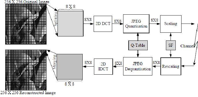
The reasons of using transforms, DFT or others, are multiple: compression, denoising, feature extraction, etc. As an example, the discrete cosine transform (DCT) is used in JPEG image compression.
NoteTransform examples
2.4.3.2 Transform example 1
Consider the exercise from Week 2:
\[x[n] = \lbrace ..., 0, \frac{1}{3}, \frac{2}{3}, 1, 1, 1, 1, 0, ... \rbrace\] Write the expression of \(x[n]\) based on the signal \(u[n]\).
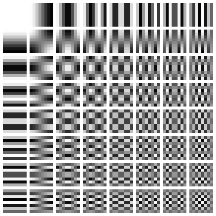
In JPEG compression, the image is divided into 8x8 blocks, and each block is transformed using the 2D Discrete Cosine Transform (DCT). This exactly corresponds to the matrix multiplication approach we discussed above, except that the basis vectors are the 64 DCT basis vectors.
The DCT transform transforms the 64 pixels of a block into 64 DCT coefficients, similar to the DFT transforming a signal of length \(N\) into \(N\) DFT coefficients.
Why? Because, unlike the 64 pixel values, out of the 64 DCT coefficients many are small negligible, and can be quantized to zero, leading to compression. When the image is reconstructed, the DCT coefficients are transformed back into pixel values using the inverse DCT, and the quantized or missing DCT coefficients not having a large effect on the image quality.
2.4.4 Properties of the DFT
2.4.4.1 Linearity
If the signal \(x_1[n]\) has the DFT coefficients \(X_k^{(1)}\), and \(x_2[n]\) has \(X_k^{(2)}\), then their sum has \[a \cdot x_1[n] + b\cdot x_2[n] \leftrightarrow a \cdot X_k^{(1)} + b\cdot X_k^{(2)} \]
Proof: via definition. Also, since DFT is equivalent to a matrix multiplication, this property is inherited from the linearity of matrix multiplication.
2.4.4.2 Shifting in time
The DFT coefficients of a signal \(x[n]\) delayed by \(n_0\) are the DFT coefficients of the original signal, multiplied by a complex exponential: If \(x[n] \leftrightarrow X_k\), then \[x[n - n_0] \leftrightarrow e^{(-j 2 \pi k n_0 / N)} X_k\]
Proof: via definition
Note that \[ | e^{(-j 2 \pi k n_0 / N)} X(\omega) | = | X(\omega) |\] which shows that when a signal is shifted in time, the amplitudes \(|X(\omega)|\) of the spectrum are not affected. Shifting in time affects only the phase of the spectrum. This makes sense, because shifting a signal in time does not change the amplitudes of the composing sinusoids, it only shifts them.
2.4.4.3 Modulation in time
A shift of the spectrum \(X_k\) by \(k_0\) corresponds to a modulation of the signal \(x[n]\) by a complex exponential:
\[e^{j 2 \pi k_0 n / N} \leftrightarrow X_{k-k_0}\]
2.4.4.4 Complex conjugation
Complex conjugation in time domain corresponds in frequency domain to complex conjugation and inversion of the frequency:
\[x^*[n] \leftrightarrow X_{-k}^*\]
2.4.4.5 Circular convolution
We define now the circular convolution of two signals \(x_1[n]\) and \(x_2[n]\) with period \(N\), which is slightly different from the normal convolution.
CIrcular convolution is similar to normal convolution, but specifically for periodic signals. Thus, it takes two periodic signals of period N (in fact, two periods of the signals), and the result is also a periodic signal of period N (one period of the result). In other words, it takes two vectors of length N and produces another vector of length N, each of these vectors being a period of a periodic signal of period N. This is different from the normal convolution, which produces a result that is longer than the original signals, i.e. a vector of length 2N.
TBD: Example at the whiteboard: how it is computed
The property of DFT is that the circular, not the linear, convolution of two signals in time domain corresponds to the product of their DFT coefficients in frequency domain: \[x_1[n] \otimes x_2[n] \leftrightarrow N \cdot X_k^{(1)} \cdot X_k^{(2)}\]
2.4.4.6 Product in time
The product of two signals in time domain corresponds to the circular convolution of their spectra in frequency domain: \[x_1[n] \cdot x_2[n] \leftrightarrow \sum_{m=0}^{N-1} X_m^{(1)} X_{(k-m)_N}^{(2)} = X_k^{(1)} \otimes X_k^{(2)}\]
2.4.4.7 Parseval theorem
The Parseval theorem states that the energy of the signal is the same in time and frequency domains: \[E = \sum_{0}^{N-1} |x[n]|^2 = \frac{1}{2 \pi} \sum |X_k|^2\]
The energy of a signal is defined as the sum of the squares of its values. Here we have two discrete set of values both in time and frequency domains, so we use the sum instead of the integral in both domains.
2.4.5 Examples of DTFT and DFT
TipExample
Let’s plot / sketch DTFT and DFT of various signals
DTFT of:
a constant signal \(x[n] = A\)
a rectangular signal \(x[n] = A\) between \(-\tau\) and \(\tau\), 0 elsewhere
a cosine of frequency precisely \(f = k/N\)
a cosine of frequency not \(f = k/N\)
DFT, with N=20, of:
a constant signal \(x[n] = A\)
a rectangular signal \(x[n] = A\) between \(-\tau\) and \(\tau\), 0 elsewhere
a cosine of frequency precisely \(f = k/N\)
a cosine of frequency not \(f = k/N\)
2.5 Relationship between DTFT and DFT
The DTFT transform is used for non-periodic signals, and produces a continuous spectrum.
The DFT transform is used for periodic signals, and produces a discrete spectrum.
We observe the fundamental duality of time and frequency, same for all Fourier transforms: a signal periodic in time has a spectrum discrete in frequency.
Discrete in one domain \(\leftrightarrow\) Periodic in the other domain
discrete in time –> periodic in frequency
periodic in time –> discrete in frequency
Continuous in one domain \(\leftrightarrow\) Non-periodic in the other domain
continous in time –> non-periodic in frequency
non-periodic in time –> continuous in frequency
Moreover, there is a close relationship between the two values of the transforms. The discrete DFT coefficients are samples of the continuous DTFT spectrum of a single period of the signal (assuming the signal is surrounded by zeros).
In general, consider a non-periodic signal \(x[n]\), from which we construct a periodic signal \(x_N[n]\) by repeating \(x[n]\) every \(N\) samples (we “periodize” \(x[n]\) with period \(N\)).
The non-periodic \(x[n]\) has a continuous spectrum \(X(\omega)\), and the periodic signal \(x_N[n]\) has \(N\) discrete DFT coefficients \(X_k\). The values of \(X_k\) are samples of the continuous spectrum \(X(\omega)\) at frequencies \(k/N\): \[X_k = X(2 \pi (k/N) n)\]
To illustrate this, consider a sequence of 7 values: \[x = [6, 3, -4, 2, 0, 1, 2]\] and let’s compute both the DTFT and DFT starting from these values.
If we consider a \(x\) surrounded by infinitely long zeros, i.e. \(x[n]\) is non-periodical, we have a continuous spectrum \(X(\omega)\) given by the DTFT: \[x_{non-per}[n] = [...0, 0, \underbrace{6, 3, -4, 2, 0, 1, 2}_{\textrm{one period}}, 0, 0, ...] \leftrightarrow X(\omega)\]
If we consider that \(x\) just one period of a periodic signal, the values repeating themselves every 7 samples: \[x_{per_7}[n] = \sum_{k=-\infty}^{\infty} x[n - 7 k]\] we can compute the DFT of this signal, based on the 7 values: \[x_{per_7}[n] = [..., -4, 2, 0, 1, 2, \underbrace{6, 3, -4, 2, 0, 1, 2}_{\textrm{one period}}, 6, 3, -4, ...] \leftrightarrow X_k \]
The values \(X_k\) are just samples from \(X(\omega)\), at taken at frequencies \(k/N\): \[X_k = X(2 \pi (k/N) n)\]
We can even repeat the 7 values with a larger period, e.g. \(N=10\), by adding zeros in between: \[x_{per_{10}}[n] = \sum_{k=-\infty}^{\infty} x[n - 10 k]\]\[x_{per_{10}}[n] = [..., 0, 6, 3, -4, 2, 0, 1, 2, 0, 0, 0, \underbrace{6, 3, -4, 2, 0, 1, 2, 0, 0, 0}_{\textrm{one period}}, 6, 3, -4, ...] \leftrightarrow X_k \]
The values \(X_k\) are still samples from \(X(\omega)\), but since \(N=10\), we have 10 samples taken at frequencies \(k/10\):
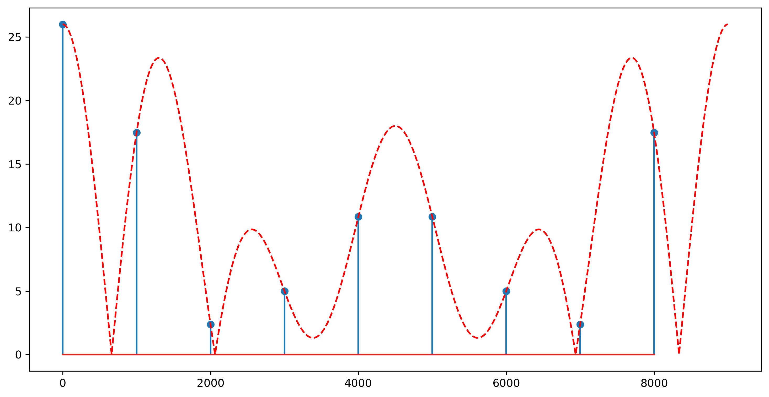
The illustration below shows this relationship, for a vector \(x = [6, 5, 4, -3, 2, -3, 4, 5, 6]\).:
The red line is the DTFT of the values \(x\), which assumes it is surrounded by zeros and forms a non-periodic signal
The blue line is the DFT of the values \(x\), which assumes they are periodic. Note that the DFT is just samples from the DTFT.
Note that in practice we can’t compute the DTFT of a signal with numerical tools like Matlab, because the DTFT is a continuous function. Instead, we can extend the signal with many zeros, and then compute the DFT of the extended signal. We will have therefore many samples of the continous spectrum, enough to plot it as a continuous function. For example, to plot the continuous spectrum of a signal \(x\) above, we extended it with zeros to a length of 10000 samples and then computed the 10000 DFT coefficients, which is achieved by the fft(x, 10000) function call in Matlab. There is no other way to compute the DTFT of a signal with numerical tools.
2.6 Signal windowing and frequency resolution
In the following, we discuss the effect of working with a finite segment of a signal, which is always the case in practice.
2.6.1 Initial example
Consider the
n=0:99;f=0.015;x=cos(2*pi*f*n)plot(abs(fft(x)))
Discuss:
Why is the spectrum not just 2 Diracs, like a normal cos()?
FFT assumes periodicity. Are there boundary problems?
What is the role of the rectangular window?
What happens if we run fft(x, 10000) instead of fft(x)?
2.6.1.1 Discussion
When we have the finite-length cosine vector \(x\), we have just a part of the signal. The true signal \(x\), infinitely long, is actually multiplied with a rectangular window \(w[n]\)\[x = cos(2 \pi f n) \cdot w[n]\].
Multiplication in time means convolution in frequency, and thus the spectrum of the true infinitely-long \(x\), i.e. two Diracs, is convoluted with the spectrum of the rectangular window, \(W(\omega)\).
Thus, the spectrum of our finite-length \(x\) is not just two Diracs, but the convolution of two Diracs with \(W(\omega)\). Thus, instead of two Diracs, we have a \(sinc()\)-like function, with a wide peak and secondary lobes.
2.6.2 Signal windowing and frequency resolution
Working with a finite-length segment of a signal always distorts its spectrum.
Suppose we have a very long, possibly infinitely-long, signal \(x[n]\) with a spectrum \(X(\omega)\).
Out of this signal, we take a segment of length \(N\), \(x_w[n]\) (for example, in order to process it with a computer).
Taking this segment is equivalent to multiplying the signal with a rectangular window \(w[n]\) of length \(N\): \[x_w[n] = x[n] \cdot w[n]\] The window \(w[n]\) can be the rectangular window, which leaves \(N\) samples unchanged and zeroes the rest, or any other window or function.
The spectrum of the windowed signal \(x_w[n]\) is the convolution of the spectrum of the original signal \(X(\omega)\) with the spectrum of the window \(W(\omega)\): \[X_w(\omega) = X(\omega) * W(\omega)\]
As a result, the spectrum of the windowed signal \(x_w[n]\) is not the same as the spectrum of the original signal \(x[n]\).
If the true signal \(x[n]\) is infinitely long, the spectrum \(X(\omega)\) is composed of just two Diracs. But if we have only a segment of the signal, which is always the case in practice, the spectrum is not just two Diracs, but a convolution of two Diracs with the spectrum of the window \(W(\omega)\). As a result, every Dirac in the spectrum of the original signal is “smudged” into a \(W(\omega)\). This is unavoidable.
Different windows \(w[n]\) have different spectra \(W(\omega)\). For example, the rectangular window has a \(sinc()\)-like spectrum, with a narrow central peak but large secondary lobes. Other windows, like the Hamming or Hann window, trade the width of the central peak with the height of the secondary lobes. However, every window \(w[n]\) will always distort the spectrum of the signal.
The only way to mitigate this effect is to work with a longer segment of the signal, which means taking more samples.
What is the problem with this? We lose frequency resolution.
Frequency resolution is the ability to distinguish between closely spaced frequency components in a signal, e.g. two Diracs close to each other.
The window spectrum \(W(\omega)\) “blurs” the spectrum of the signal. We are looking at the spectrum through a “blurred lens” \(W(\omega)\). For example, two close Diracs are be impossible to differentiate, because the “blur” will change them into overlapping peaks, which we can’t separate. Secondary lobes of the window \(W(\omega)\) will mask other Diracs in the spectrum, smaller but further away.
In short, working with a finite-length segment of a signal always distorts its spectrum. Having a short segment of a signal leads to low frequency resolution, because the spectrum is “blurred” by the window. The only way to increase frequency resolution is to work with a longer segment of the signal, which means taking more samples. Frequency resolution is proportional to the length of the segment.
There are many windows available, each with different spectra \(W(\omega)\).
Recangular window
Hamming window
Hann window
…
The rectangular window has the narrowest central peak, but the largest secondary lobes. Other windows have wider central peaks, but smaller secondary lobes. They can be useful to attenuate sharp transitions at the boundaries of the signal, thus reducing the boundary problems.
NoteRemember
Every time we work with a piece of a signal (for example we process an audio file working on segments of 1024 samples), we are applying windowing, and this distorts the spectrum.
Even the rectangular window is still a window. Always consider if it is useful to replace the rectangular window with another one, especially if you use fft() or other frequency-based operations (hint: most often it is).
2.7 STFT and Spectrograms
How can we analyze the frequency of a signal whose frequency components change in time (e.g. like a musical song)?
The Short-Time Fourier Transform (STFT) is a a technique for analyzing the frequency content of local sections of a signal as it changes over time.
STFT divides a longer time signal into shorter segments of equal length and then computes the Fourier Transform separately on each short segment:
Split the signal into pieces (e.g. 1024-samples long), possibly overlapping
Compute the spectrum of every piece (e.g. fft())
Display the resulting sequence of spectra as an image, known as a spectrogram.
The STFT is a time-frequency representation of a signal, because the resulting spectrogram is 2D, with two axes: time and frequency.
It is common for the segments to overlap, e.g. 10% overlap, in order to have a smoother transition between segments.
The STFT depends on two parameters:
The length of the segments (e.g. 1024 samples)
The overlap between segments (e.g. 10%)
The length of the segments affects the time resolution and the frequency resolution of the spectrogram.
If the segments have short length, we have good time resolution, because we can pinpoint the moment in time where a frequency component appears with high precision. However, we have poor frequency resolution, because the spectrum of a short segment is more “blurred”
If the segments have long length, we have poor time resolution, because we can’t pinpoint the moment in time where a frequency component appears with high precision, but we have good frequency resolution, because the spectrum of a long segment is less “blurred”.
This illustrates the Time-frequency Uncertainty Principle, which states that you cannot have very good time resolution and very good frequency resolution simultaneously. This principle is often encountered in many areas of engineering, physics, or mathematics.
A small overlap between segments is useful to have a smoother transition between segments, and avoid hard-splitting a frequency component between two adjacent segments. Common values range from 10% to 50%.
2.8 Geometric interpretation of Fourier Transform (DTFT)
Consider a signal \(x[n]\) with the Z-transform \(X(z)\), with zeros \(z_1, z_2, \dots\) and poles \(p_1, p_2, \dots\): \[X(z) = C \cdot \frac{(z-z_1)\cdots(z - z_M)}{(z-p_1)\cdots(z - p_N)}\]
The DTFT is: \[X(\omega) = C \cdot \frac{(e^{j \omega}-z_1)\cdots(e^{j \omega} - z_M)}{(e^{j \omega}-p_1)\cdots(e^{j \omega} - p_N)}\] with its modulus function being: \[|X(\omega)| = |C| \cdot \frac{|e^{j \omega}-z_1|\cdots|e^{j \omega} - z_M|}{|e^{j \omega}-p_1|\cdots|e^{j \omega} - p_N|}\] and phase: \[\angle{X} = \angle{C} + \angle (e^{j \omega}-z_1) + \cdots + \angle(e^{j \omega} - z_M) - \angle(e^{j \omega}-p_1) - \cdots - \angle(e^{j \omega} - p_N)\]
For any complex numbers \(a\) and \(b\), we have:
modulus of \(|a - b|\) is the length of the segment between \(a\) and \(b\)
phase of \(|a - b|\) is the angle of the segment from \(b\) to \(a\) (direction is important)
So, for a point on the unit circle \(z = e^{j \omega}\), we have:
the modulus \(|e^{j \omega} - z_k|\) or \(|e^{j \omega} - p_k|\) is the distance of that point from the zero or pole \(z_k\) or \(p_k\)
phase of \(|e^{j \omega} - z_k|\) or \(|e^{j \omega} - p_k|\) is the angle of the segment from the zero or pole to that point
As such, we can say that the modulus of the DTFT \(|X(\omega)|\), for a certain value of \(\omega\), is given by the distances to the zeros and to the poles, and the phase of the DTFT \(\angle{X(\omega)}\) is given by the angles of segments from the zeros and poles to that point.
TBD: Add figures
Consequences:
when a pole is very close to unit circle, the DTFT is large around this point (around that value of \(\omega\))
when a zero is very close to unit circle, the DTFT is small around this point (around that value of \(\omega\))
Examples: …
This geometric interpretation ignores the constant \(C\) in front of the Z-transform, which is not visible in the pole-zero plot. The value of \(|C|\) and \(\angle{C}\) must be determined separately, from another information (for example, the value of the transform at a certain point).
NoteIntuition
We can think of the Z transform \(X(z)\) as a landscape, with poles being mountains (of infinite height) and zeros being valleys (of zero height). and zeros being valleys.
The DTFT \(X(\omega)\) is like a walk over this landscape along the unit circle. The height profile of the walk gives the modulus of the Fourier transform.
When close to a mountain, the road is high, and the Fourier transform has large amplitude
When close to a valley, the road is low, and the Fourier transform has small amplitude
This allows to quickly understand and possibly sketch the shape of the Fourier Transform of a signal, just by looking at the pole-zero plot.
2.9 Terminology
Based on the frequency content of signals, we can classify them in various categories:
low-frequency signals
mid-frequency signals
high-frequency signals
Band-limited signals are signals that have all the spectrum within a certain frequency band. e.g. no larger than a frequency \(f_{max}\), and zero elsewhere.
The bandwitdh\(B\) of a signal is the frequency interval [\(f_1\), \(f_2\)] which contains \(95\%\) of energy. The size of the bandwidth is \(B = f_2 - f_1\).
Based on bandwidth \(B\), we can define the central frequency\(F_c = \frac{f_1 + f_2}{2}\), and classify signals in:
Narrow-band signals: their bandwidth \(B\) is much smaller than the central frequency \(F_c\)\[B << F_c\]
Wide-band signals: signals which are not narrow-band
2.10 Numerical examples
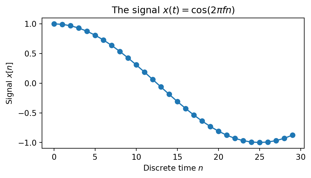
2.10.1 A sinusoidal signal
Consider a cosine signal: \[x(t) = \cos(2 \pi f n)\] with \(f = 0.01\)
This is how the signal looks like:
# Create the signalf =0.02N =30#fmax = fmax * (N-10)/Nn = np.arange(N)x = np.cos(2*np.pi*f*n)# Plot the signalplt.figure(figsize=(6, 3))plt.plot(x, '-o')plt.title('The signal $x(t) = \cos(2 \pi f n)$')plt.xlabel('Discrete time $n$')plt.ylabel('Signal $x[n]$')plt.show()
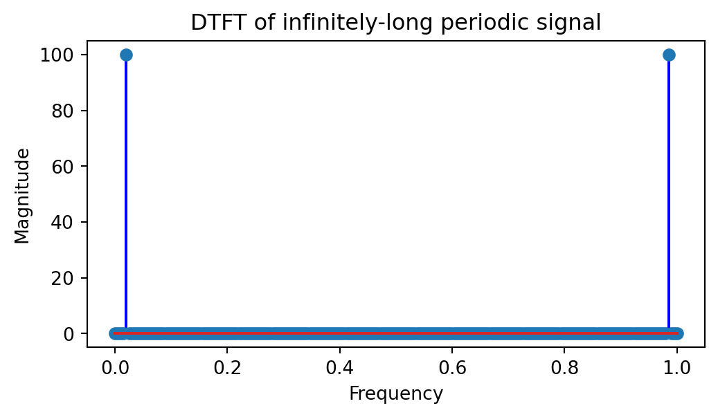
Now let’s compute the Discrete-Time Fourier transform. This assumes that the signal is infinitely long.
If the cosine signal would be infinitely long, the DTFT contains only two Dirac impulses at the corresponding frequency.
# Regenerate the signal so that it fits in one periodperiod =10000*fninf = np.arange(period)xinf = np.cos(2*np.pi*f*ninf)# Compute the DTFTSinf = fft(xinf)# Create the frequency axisfreqinf = np.linspace(fmin, fmax, len(Sinf))# Plot the magnitude of the DTFTplt.figure(figsize=(6, 3))plt.title('DTFT of infinitely-long periodic signal')plt.stem(freqinf, np.abs(Sinf), linefmt='b')plt.xlabel('Frequency')plt.ylabel('Magnitude')plt.show()
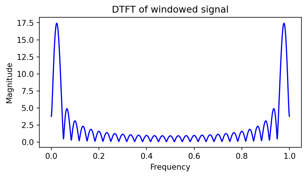
If the signal is assumed to be only the segment we defined, and is surrounded by infinitely-long zeros, i.e. a truncated cosine, then the spectrum is convoluted with the spectrum of a rectangular window, and the DTFT looks as follows:
# Compute the DTFTFFT_points =10000*n.sizeS1 = fft(x, FFT_points)# Create the frequency axisfreq1 = np.linspace(fmin, fmax, len(S1))# Plot the magnitude of the DTFTplt.figure(figsize=(6, 3))plt.title('DTFT of windowed signal')plt.plot(freq1, np.abs(S1), 'b')#plt.stem(freqinf, np.abs(Sinf), 'b')plt.xlabel('Frequency')plt.ylabel('Magnitude')plt.show()
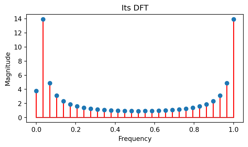
When computing the Discrete Fourier Transform (DFT), this assumes that the given piece of the signal is would be repeated periodically. The DFT is not continous, it is discrete.
# Compute the DFTS2 = fft(x)# Create the frequency axisfreq2 = np.linspace(fmin, fmax, len(S2))#freq2 = np.fft.fftfreq(x.size)# Plot the magnitude of the DTFTplt.figure(figsize=(6, 3))plt.title('Its DFT')plt.stem(freq2, np.abs(S2), linefmt='ro')plt.xlabel('Frequency')plt.ylabel('Magnitude')plt.show()
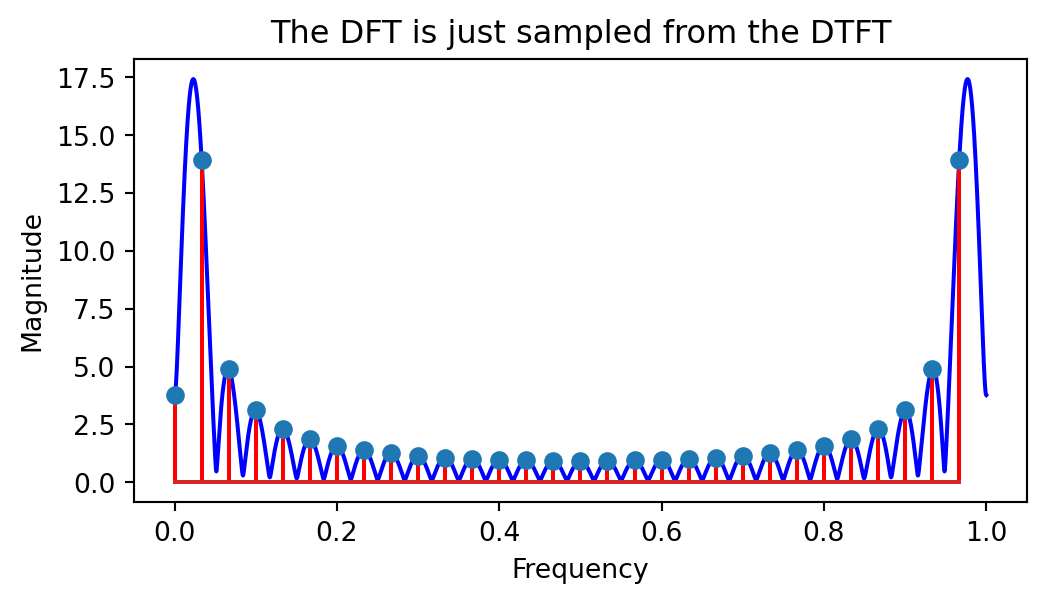
The DFT is just sampled from the DTFT:
# Plot the DTFT and DFT overlaidfreq2 = np.linspace(fmin, fmax, len(S2)+1)plt.figure(figsize=(6, 3))plt.plot(freq1, np.abs(S1), 'b')plt.stem(freq2[:-1], np.abs(S2), linefmt='ro')plt.title('The DFT is just sampled from the DTFT')plt.xlabel('Frequency')plt.ylabel('Magnitude')plt.show()
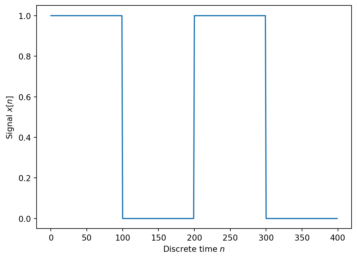
2.10.2 A rectangle pulse
Consider a rectangle pulse signal as below:
# Create the signallen_1 =100len_0 =100x = np.hstack((np.ones(len_1), np.zeros(len_1)))x = np.hstack((x, x))# Plot the signalplt.figure()plt.plot(x)plt.xlabel('Discrete time $n$')plt.ylabel('Signal $x[n]$')plt.show()
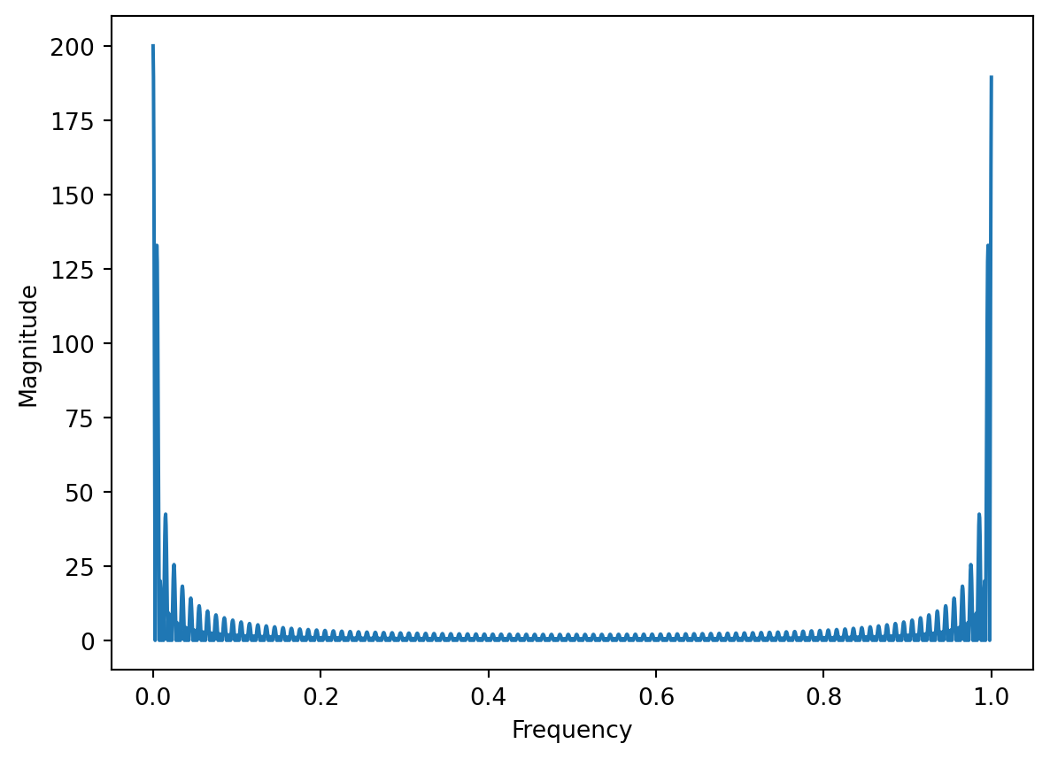
The DTFT is:
# Compute the DTFT of the rectangle windowFFT_points =2000W = fft(x, FFT_points)# Create the frequency axisfreq = np.linspace(fmin, fmax, len(W))# Plot the magnitude of the DTFTplt.figure()plt.plot(freq, np.abs(W))plt.xlabel('Frequency')plt.ylabel('Magnitude')plt.show()
image from: JPEG Picture Compression Using Discrete Cosine Transform, N. K. More, S. Dubey, 2012↩︎