Source Coding¶

In this chapter we take a look at the basic principles and algorithms for data compression.

1The role of coding¶

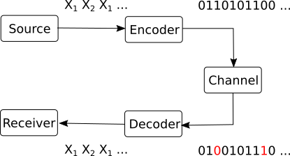
In the general block diagram of a communication system, the coding block is situated between the information source and the communication channel.

Communication system {width=35%}

It’s role is to prepare the raw information in order to be transmitted over the channel. It has two main jobs:

Source coding:
- Convert source messages to channel symbols, i.e. the actual symbols which the channel knows to transmit.
  For example, express the messages in binary form (zeros and ones), for sending over a binary channel.
- Minimize the number of symbols needed to be transmitted (i.e., data compression). We don’t want to transmit more symbols than necessary to recover the messages at the receiving end.
- Adapt probabilities of symbols in order to maximize to maximize mutual information. We will discuss this more in Chapter IV.
Error control coding
- Protect the information against channel errors
- Also known as “channel coding”

Basically, source coding refers to all the procedures required to express the source messages as channel symbols in the most efficient way possible, while error control coding refers to all the algorithms used to protect the data against errors.

The coding block has a corresponding decoding block on the receiving end. Its job is to “undo” all the coding operations:

detect and fix the errors in the received data, based on the algorithms introduced by the coding block
convert the channel symbols back into the message representations that the receiver expects

Is it possible to do these two jobs separately, one after another, in two consecutive operations? Yes, as the source-channel separation theorem establishes.

We give below only an informal statement of the theorem:

In this chapter, we consider only the source coding algorithms, without any error control. Basically, we assume that data transmission is done over an ideal channel with no noise, and therefore the transmitted symbols are perfectly recovered at the receiver.

In this context, our main concern is how to minimize the number of symbols needed to represent the messages, while making sure that the receiver can decode the messages correctly. The advantages of data compression are self-evident:

Efficiency
Short communication times
Can decode easily

2Definitions¶

Let’s define what coding means from a mathematical perspective.

Consider an input information source with the set of messages:

S = \left\lbrace s_1, s_2, ... s_N \right\rbrace

(1)

and suppose we would like to express the messages as a sequence of the following code symbols:

X = \left\lbrace x_1, x_2, ... x_M \right\rbrace

(2)

The set $X$ is known as the alphabet of the code.

For example, for a binary code we have $X = \lbrace 0, 1\rbrace$ and a possible sequence of symbols is $c = 00101101$

Definition 1 (Code definition)

A code is a mapping from the set $S$ of $N$ messages to a set of $N$ sequences of symbols, known as codewords:

C = \left\lbrace c_1, c_2, ... c_N \right\rbrace

(3)

An example code mapping is given below:

Message		Codeword
$s_1$	$\rightarrow$	$c_1 = x_1x_2x_1...$
$s_2$	$\rightarrow$	$c_2 = x_1x_2x_2...$
$\dots$	$\rightarrow$	$\dots$
$s_N$	$\rightarrow$	$c_N = x_2x_2x_2...$

The codewords are the sequences of symbols used by the code.

The codeword length, which we denote as $l_i$ , is the the number of symbols in a given codeword $c_i$ .

Encoding a given message or sequences of messages means replacing each message with its codeword.

Decoding means deducing back the original sequence of messages, given a sequence of symbols.

As an example, the ASCII code is a widely-used code for encoding characters, consisting of 256 codewords (stored on 1 byte):

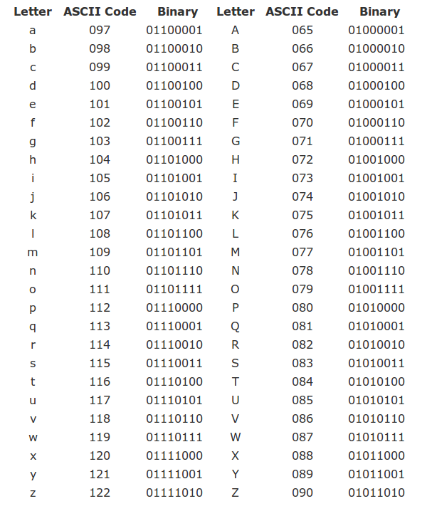
Nowadays, ASCII is usually replaced by Unicode (UTF-8), which is a more general code using 65536 codewords (stored on 2 bytes), allowing for many more letters used in languages around the globe.

2.1The graph of a code¶

The codewords of a code can represented as a binary tree. We call this representation the graph of the code.

TODO: Example at blackboard

2.2Average code length¶

There are many ways to define the codewords for messages, but some are better than others.

The most basic quantity indicating efficiency of a code is the average code length.

For every codeword $c_i$ , we multiply the probability of the corresponding message $p(s_i)$ with its length $l_i$ .

A code with smaller average length is better, because it represents sequences of messages with less symbols, on average. However, there is a certain lower limit to how small the average length can be (for example, it cannot be 0, for self-evident reasons).

This raises the following interesting question:

Given a source $S$ , how small can the average length be?

This is a fundamental question, to which we will provide an answer later in this chapter.

2.3Instantaneous codes¶

We introduce another set of useful definitions regarding the codeword structure.

A code can be:

non-singular: all codewords are different
uniquely decodable: no two sequences of messages translate to the same sequence of symbols
- i.e. there is never a confusion at decoding: there can be only one sequence of messages corresponding to a given sequence of symbols
instantaneous (also known as prefix-free): no codeword is prefix to another code
- A prefix = a codeword which is the beginning of another codeword

Examples: at the blackboard

The follwing relations exist between these types of codes.

We can summarize the relation between these three code types as follows:

Instantaneous $\subset$ uniquely decodable $\subset$ non-singular

Graph-based decoding of instantaneous codes¶

Using the graph of the code, we can use a very simple procedure for decoding any instantaneous code:

TODO: TBD: Illustrate at whiteboard

This procedure shows the advantage of instantaneous codes over other codes which might be uniquely decodable, but are not instantaneous. Instantaneous codes allow for simple decoding. There is never any doubt about the next message in the sequence.

This decoding scheme is also showing why these codes are named “instantaneous”: a codeword can be decoded as soon as it is fully received, immediately, without any delay, because the decoding takes place on-the-fly while the bits are received one-by-one.

As a counter example, consider the following uniquely decodable, but non-instantaneous code: $\left\lbrace 0, 01, 011, 1110 \right\rbrace$ . When you read the first 0, you cannot decode it yet, because you need to wait the next bits to understand how to segment the sequence. This implies that the decoding has some delay.

3The Kraft inequality theorem¶

When can an instantaneous code exist? Given a DMS $S$ , are we sure we can find an instantaneous code for it, and if yes, under which conditions?

The answers to these questions is provided by the Kraft inequality.

Comments on the Kraft inequality:

If lengths do not satisfy the relation, no instantaneous code exists with these lengths
If the lengths of a code satisfy the relation, that code can be instantaneous or not (there exists an instantaneous code, but not necessarily that one). Keep in mind that the Kraft inequality only looks at the lengths of the codewords, not at their actual symbols, so it can only say something about the lengths, not about the actual codewords
The Kraft inequality implies that the codewords lengths cannot be all very small, because if all $l_i$ values are too small the sum exceeds 1. Thus, implicitly, it sets a lower limit to the permissible lengths.
From the proof, it follows that we have equality in the relation
$\sum_i D^{-l_i} = 1$
(6)
only if the lowest level of the tree is fully covered. Thus, for an instantaneous code which satisfies Kraft with equality, all the graph branches terminate with codewords and there are no unused branches.
This makes sense intuitively, since is most economical way: codewords are as short as they can be. Any unused branch means that we can actually make the code shorter by moving some message up the tree.

We have seen that instantaneous codes must obey the Kraft inequality But how about uniquely decodable codes? The answer is given by the next theorem.

Consequences of the McMillan theorem:

For every uniquely decodable code, there exists in instantaneous code with the same lengths. This is because the lengths $l_i$ must satisfy the same relation both for unique-decodable and for instantanous codes.
Thus, even though the class of uniquely decodable codes is larger than that of instantaneous codes (because any instantaneous code is uniquely decodable, but not any uniquely decodable code is instantaneous), using uniquely-decodable codes brings no additional benefit in average codeword length
Instead of an uniquely decodable code, we can always use an instantaneous code, which has the same lengths, but is much easier to decode.

3.1Finding an instantaneous code for given lengths¶

How to find codewords with code lengths $\{l_i\}$ ?

In general, we may use the following procedure:

Note that this procedure only gives us the codewords, not the mapping to a particular set of messages.

In practice, there might be more elaborate ways to find the codewords and map them to the messages of the source, with additional benefits.

4Minimum average length¶

We will discuss now one of the most important aspect of this chapter,

Given a DMS $S$ , suppose we want to find an instantenous code for it, but in such a way as to minimize the average length of the code:

\overline{l} = \sum_i p(s_i) l_i

(8)

How can we find such an optimal code?

Given that it should be instantaneous, the codeword lengths must obey the Kraft inequality.

In mathenatical terms, we formulate the problem as a constrained optimization problem:

\begin{aligned} \textbf{minimize } &\sum_i p(s_i) l_i \\ \textrm{subject to } &\sum_i D^{-l_i} \leq 1 \end{aligned}

(9)

This means that we want to find the unknowns $l_i$ in order to minimize a certain quantity ( $\sum_i p(s_i) l_i$ ), but the unknowns must satisfy a certain constraint ( $\sum_i D^{-l_i} \leq 1$ ).

4.1The method of Lagrange multipliers¶

To solve this problem, we use a standard mathematical tool known as the method of Lagrange multipliers.

Definition 3 (Lagrange multipliers for constrained optimization problems)

To solve the following constrained optimization problem:

\begin{aligned} \textbf{minimize } & f(x) \\ \textrm{subject to } & g(x) = 0 \end{aligned}

(10)

one must build a new function $L(x, \lambda)$ (known as the Lagrangean function):

L(x, \lambda) = f(x) - \lambda g(x)

(11)

The solution $x$ of the original problem is among the solutions of the system:

\begin{cases} \frac{\partial L(x, \lambda)}{\partial x} &= 0 \\ \frac{\partial L(x, \lambda)}{\partial \lambda} &= 0 \end{cases}

(12)

If there are multiple variables $x_i$ in the problem, we take the partial derivative $\frac{\partial L(x, \lambda)}{\partial x_i}$ for each one of them, resulting in a larger system.

Let’s use this mathematical formulation to our problem. In our case, the functions and the variables involved are the following:

The unknowns $x_i$ are the lengths $l_i$
The function to minimize is $f(x) = f(l_i) = \overline{l} = \sum_i p(s_i) l_i$
The constraint is $g(x) = g(l_i) = \sum_i D^{-l_i} - 1$

The resulting optimal codeword lengths are:

l_i = -\log(p(s_i))

(16)

Proof 5

We use the Lagrange multpliers method to solve the following optimization problem:

\begin{aligned} \textbf{minimize } &\sum_i p(s_i) l_i \\ \textrm{subject to } &\sum_i D^{-l_i} = 1 \end{aligned}

(18)

which is an instance of the general constrained optimization problem:

\begin{aligned} \textbf{minimize } & f(x) \\ \textrm{subject to } & g(x) = 0 \end{aligned}

(19)

with $f(x) = \sum_i p(s_i) l_i$ and $g(x) = \sum_i D^{-l_i} - 1$ .

The Lagrangean function is:

L(x, \lambda) = f(x) - \lambda g(x) = \sum_i p(s_i) l_i - \lambda \left( \sum_i D^{-l_i} - 1 \right)

(20)

We derivate the Lagrangean function with respect to all $l_i$ and the $\lambda$ , and set the results to zero:

\begin{cases} \frac{\partial L(x, \lambda)}{\partial l_i} &= 0, \forall i=1...N \\ \frac{\partial L(x, \lambda)}{\partial \lambda} &= 0 \end{cases}

(21)

The second equation gives us:

\frac{\partial L(x, \lambda)}{\partial \lambda} = \sum_i D^{-l_i} - 1 = 0 \Rightarrow \sum_i D^{-l_i} = 1

(22)

which is just the Kraft constraint.

The first equation gives us:

\frac{\partial L(x, \lambda)}{\partial l_i} = p(s_i) + \lambda \ln(D) D^{-l_i} = 0,\qquad \forall i=1...N

(23)

These are actually $N$ equations, one for each variable $l_i$ . Summing all of these equations, we obtain:

\sum_i p(s_i) + \lambda \ln(D) \sum_i D^{-l_i} = 0

(24)

and since $\sum_i p(s_i) = 1$ and $\sum_i D^{-l_i} = 1$ , we obtain:

1 + \lambda \ln(D) = 0 \Rightarrow \lambda = -\frac{1}{\ln(D)}

(25)

Plugging this value back into each of the first equations, we obtain

p(s_i) -\frac{1}{\ln(D)} \ln(D) D^{-l_i} = 0

(26)

which leads to the optimal codeword lengths:

l_i = -\log_D(p(s_i))

(27)

In particular, for binary codes ( $D=2$ ), the optimal codeword lengths are:

l_i = -\log_2(p(s_i))

(28)

The fundamental interpretation of this result is that, in order to minimize the average length of a code, a message with higher probability must have a shorter codeword, while a message with lower probability must have a longer codeword. This makes sense because messages we can afford to use a longer codeword for messages which appear rarely in a sequence.

4.2Entropy is the limit¶

Another fundamental consequence of the preceding theorem gives us a functional definition of the entropy, i.e. it tells us what the entropy really says about an information source.

Assume we have a binary code (we choose it binary in order to match the choice of $\log_2()$ in the definition of entropy).

Since the optimal codeword lenghts are $l_i = -\log_2(p(s_i))$ , then the minimal average length obtainable is equal the entropy of the source:

\min \overline{l} = \sum_i p(s_i) {l_i}_{min} = -\sum_i p(s_i) \log(p(s_i)) = H(S)

(29)

This result tells us what the entropy really means, besides the algebric definition provided in chapter I. The entropy gives us the minimum number of bits required to represent the data generated by an information source in binary form. Although we rigorously proved this result only for a discrete memoryless source, it holds for sources with memory as well.

Some immediate consequences:

Messages from a source with small entropy can be written (encoded) with few bits
A source with with large entropy requires more bits for encoding the messages

Reformulating this in a different way, we can say that he average length of an uniquely decodable code must be at least as large as the source entropy. One can never represent messages, on average, with a code having average length less than the entropy.

H(S) \leq \overline{l}

(30)

Efficiency and redundancy of a code¶

Considering a code for an information source, comparing the average code length with the entropy indicates the efficiency of the encoding. These quantities indicate how close is the average length to the optimal value.

Coding with the wrong code¶

An interesting question arises in practice. Consider a source with probabilities $q(s_i)$ . We design a code for this source, but we use it to encode messages from a different source, with probabilities $p(s_i)$ .

This happens in practice when we estimate the probabilities from a sample data file, and then we use the code for general of similar files. Those files might not have exactly the same frequencies of messages as the sample file used to design the code.

How does this affect us? We lose some efficiency, because the codeword lengths $\overline{l_i} \approx -\log_2(q_i)$ are not optimal for the source with probabilities $p_i$ , which leads to increased average length.

If the codewords were optimal, the codeword lengths would have been $\approx -log_2(p_i)$ , leading to an average length equal to the entropy $H(S)$ :

\overline{l_{optimal}} = -\sum{p(s_i) \log{p(s_i)}}

(33)

But the actual average length we obtain is:

\overline{l_{actual}} = \sum{p(s_i) l_i} = -\sum{p(s_i) \log{q(s_i)}}

(34)

The difference between average lengths is what we lose due to the mismatch:

\overline{l_{actual}} - \overline{l_{optimal}} = \sum_i{p(s_i) \log(\frac{p(s_i)}{q(s_i)})} = D_{KL}(p || q)

(35)

The difference is exactly the Kullback-Leibler distance between the two distributions $p$ and $q$ .

Therefore we have a functional definition of the KL distance: the KL distance between two distributions $p$ and $q$ is the number of extra bits spent when we encode messages from $p$ using a code optimized for a different distribution $q$ .

Due to the KL distance properties, the distance is always $\geq 0$ , which shows that such a mismatch always increases the average length. The more different the two distributions are, the larger the increase in average length becomes.

5Coding procedures¶

5.1Optimal and non-optimal codes¶

A code for which $\eta = 1$ is known as an optimal code. Such a code attains the minimum average length:

\overline{l} = H(S)

(36)

However, this is only possible if the probabilities are powers of 2, such that $l_i = -log2(p(s_i))$ is an integer number, because the codeword lengths must always be natural numbers.

e.g. probabilities like $1/2$ , $1/4$ , $1/2^n$ , known as dyadic distribution
the lengths $l_i = -\log(p(s_i))$ are all natural numbers

An optimal code can always be found for a source where all $p(s_i)$ are powers of 2, using for example the graph-based procedure explained earlier.

However, in the general case $l_i = -\log(p(s_i))$ might not be an integer number. This happens when $p(s_i)$ is not a power of 2. What to do in this case?

A simple solution to this problem is to round every logarithm to next largest natural number:

l_i = \lceil -\log(p(s_i)) \rceil

(37)

for example:

-\log(p(s_i)) = 2.15 => l_i = 3

(38)

This leads to the Shannon coding algorithm described below.

5.2Shannon coding¶

The Shannon coding procedure is a simple algorithm for finding an instantaneous code for a DMS.

The code obtained with this procedure is known as a Shannon code.

Shannon coding is one of the simplest algorithms, and some other better schemes are available. However, this simplicity allows to prove fundamental results in coding theory, as we shall see below.

One such fundamental result shows that the average length of a Shannon code is actually close to the entropy of the source.

Proof 6

The first inequality, $H(S) \leq \overline{l}$ , is because $H(S)$ is the minimum average length.

To prove the second inequality, consider the lenghts $l_i$ obtained with the Shannon algorithm:

l_i = \lceil -\log(p(s_i)) \rceil = -\log(p(s_i)) + \epsilon_i

(41)

where the values are rounded upwards with a quantity $\epsilon_i$ which is smaller than 1, $0 \leq \epsilon_i < 1$ .

Computing the average length, we have:

\begin{aligned} \overline{l} &= \sum_i p(s_i) l_i \\ &= \sum_i p(s_i) (-\log(p(s_i)) + \epsilon_i) \\ &= H(S) + \underbrace{\sum_i p(s_i) \epsilon_i}_{< 1} \\ &\leq H(S) + \sum_i p(s_i) \cdot 1 \\ &= H(S) + 1 \end{aligned}

(42)

We have used the fact that $\epsilon_i < 1$ , which makes the sum $\sum_i p(s_i) \epsilon_i$ smaller or equal to $\sum_i p(s_i)$ , which is 1.

Although a Shannon code is not optimal, in the sense that it does not lead to the minimum achievable average length, we see that it’s also not very bad. The average length of Shannon code is at most 1 bit longer than the minimum possible value, which is quite efficient. However, better procedures do exist.

5.3Shannon’s first theorem¶

Shannon’s first theorem (coding theorem for noiseless channels) shows us that, in theory, we can approach the entropy as close as we want, using extended sources.

Proof 7

First, note that the average length can never go below H(S), because this is minimum. We only consider getting close to H(S) from above.

Let’s consider the $n$ -th order extension $S^n$ of the source S.

$S^n$ is a source like any other, with its own probabilities $p(\sigma_i)$ , and it can undergo Shannon coding as well. When we use Shannon coding for $S^n$ , it satisfies the same condition:

H(S^n) \leq \overline{l_{S^n}} < H(S^n) + 1

(43)

where $\overline{l_{S^n}}$ is the average length of the codewords for $S^n$ .

We have $H(S^n) = n H(S)$ , due to the theorem for extended sources.

Because a message of $S^n$ is just a group of $n$ messages of $S$ , we have the average length per message of $S$ as:

\overline{l_{S}} = \frac{\overline{l_{S^n}}}{n}

(44)

Therefore, dividing by $n$ , we obtain:

\boxed{H(S) \leq \overline{l_{S}} < H(S) + \frac{1}{n}}

(45)

which means that the average length used for a message of the original source $S$ is at most $1/n$ away from the entropy $H(S)$ .

At the limit, if we consider the extension order $n \to \infty$ , we have:

\overline{l_{S}} \to H(S)

(46)

The theorem shows that, in principle, we can always obtain $\overline{l} \to H(S)$ , if we consider longer and longer sequences of messages from the source, modeled as larger and larger extensions of the source.

However, this result is mostly theoretical, because in practice the size of $S^n$ gets too large for large $n$ . Other (better) algorithms than Shannon coding are used in practice to approach $H(S)$ .

5.4Shannon-Fano coding (binary)¶

The Shannon-Fano (binary) coding procedure is presented below.

It’s easier to understand the Shannon-Fano coding by looking at an example at the whiteboard, or at a solved exercise.

Shannon-Fano coding does not always produce the shortest code lengths, but in general it is better than Shannon coding in this respect.

As a remark, there is a clear connection between Shannon-Fano coding and the optimal decision tree examples from the first chapter (with yes-no answers). Splitting the messages into two groups is similar to splitting the decision tree into two branches.

5.5Huffman coding (binary)¶

Huffman coding produces a code with the smallest average length (better than Shannon-Fano). It can be proven (though we won’t give the proof here) that no other algorithm which assigns a separate codeword for each message can produce a code with smaller average length than Huffman coding. Some better algorithms do exist, but they work differently: they do not assign a codeword to every single message, instead they code a whole sequence at once.

Assigning 0 and 1 in the backwards pass can be done in any order. This leads to different codewords, but with the same codeword lengths, so the resulting codes are equivalent.

When inserting a sum into an existing list, it may be equal to another value(s), so we may have several options where to insert: above, below or in-between equal values. This leads to codes with different individual lengths, but same average length. In general, if there are several options available, it is better to insert the sum as high as possible in the list, because this leads to a more balanced tree, and therefore the codewords tend to have more equal lengths. This is helpful in practice in things like buffering. Inserting as low as possible tends to produce codewords with more widely varying lengths, which increases the demands on the buffers.

5.6Huffman coding (M symbols)¶

All coding procedures can be extended to the general case of $M$ symbols $\left\lbrace x_1, x_2, ... x_M \right\rbrace$ . We illustrate here the generalization for Huffman coding.

Procedure:

Arrange the probabilities in descending order
Forward pass:
- Add together the last $M$ symbols, insert the sum into the list etc.
- Important: at the final step must have $M$ remaining values. It maybe necessary to add virtual messages with probability 0 at the end of the initial list, in order to end up with exactly $M$ messages in the last step.
Backward pass:
- Assign all $M$ symbols $\left\lbrace x_1, x_2, ... x_M \right\rbrace$ to each of the final $M$ messages, then go back step by step.

Example : blackboard

5.7Probability of symbols¶

Given a code $C$ with symbols $x_i$ , we can compute the probability of apparition of each symbol in the code.

The average number of apparitions of a symbol $x_i$ is:

\overline{l}_{x_i} = \sum_i p(s_i) l_{x_i}(s_i)

(48)

where $l_{x_i}(s_i)$ is number of symbols $x_i$ in the codeword of $s_i$ (e.g. the number of 0’s and 1’s in a binary codeword)

If we divide this to the average length of the code, $\overline{l}$ , we obtain the probability of symbol $x_i$ :

p(x_i) = \frac{\overline{l}_{x_i}}{\overline{l}}

(49)

These are the probabilities of the input symbols for the transmission channel, which play an important role in Chapter IV (transmission channels).

6Source coding as data compression¶

Many times, the input messages are already written in a binary code, such as the ASCII code for characters.

In this case, source coding can be understood as a form of data compression, by replacing the original binary codewords with different ones, which are shorter on average, thus using fewer bits in total to represent the same information.

This process is similar to removing predictable or unnecessary bits from a sequence, We thus reducing the redunancy of the original data. The resulting compressed data appear random and patternless.

To obtain the original data back, the decoder must undo the coding procedure. If there were no errors during the transmission, the original data is recovered exactly. This makes it a lossless compression method.

As a final note, we mention that other coding methods do exist beyond Huffman coding, which provide better results (arithmetic coding) or other advantages (adaptive schemes).