Discrete Information Sources
1A mathematical definition of information
In order to analyze information generation, encoding and transmission with mathematical tools, we need a solid and clear definition of information.
So, what is information?
Let’s start first with a simple example. Imagine someone rolls a dice and tells you the resulting value:
“The value is 5”
Does this message carry information? How, why, how much?
When thinking about the information brought by such a phrase, let’s consider the following principles:
The message carries information only when you don’t already know the result. If you already known the result, the message is useless, which means it brings zero information.
If the result was to be expected, there is little information, e.g. suppose the message is “The value is smaller than 7”. Does this carry any information?
Conversely, if the result is highly unusual, there is more information in this message
All this suggests that the information is related to the probability of some event happening, in a inverse manner: the lower the probability, the higher the information.
1.1Definition of information
Throughout this class, we refer to a probabilistic event as a “message”
Consider a message (event) which happens with probability . The information attached to is rigorously defined as:
Consequences of this definition:
Information of an event is always non-negative:
Lower probability (rare events) means higher information
Higher probability (frequent events) means lower information
The certain event ( brings no information:
An event with probability 0 brings infinite information (but it never happens...)
When two independent and events take place, their information gets added:
The information is a purely abstract mathematical quantity, and it is not related to the meaning of the message, and neither to its particular form. It’s not related to the fact that the message is written as a sentence in English, or in some other language or different signs. The information attached to an event simply states that “this event happened”, and depends only on the probability of that event.
Encoding the information as a particular sequence of symbols (letters, bits etc.) is a different matter, and shall be discussed in later chapters.
1.2Choice of logarithm
Using the logarithm function in the definition is crucial, since it is responsible for most of these properties. In particular, the fact that logarithm transforms a product into a sum allws to sum the information of independent events.
The choice of logarithm base is merely a convention. Any base of logarithm can be used in the definition, not just base 2, and all the consequences still hold.
By convention, we typically use the binary logarithm . In this case, the information is measured in bits
We could use instead the natural logarithm , and the result is measured in nats.
The choice of the algorithm is not critical and doesn’t change anything fundamental, since logarithm bases can always be converted to/from one another:
This means that information defined using different logarithms differ only by a scaling factor:
Following the convention of the scientific literature, we shall use the base 2 logarithm from now on.
1.3Information Sources
A probabilistic event is always part of a set of multiple events, containing all the possible outcomes which can happen at a given time. Continuing the previous example, the value we obtained was 5, but we could have obtained any interger between 1 and 6. There are 6 messages, each having its own probability, all known beforehand. At a given time, only one of the events can happen, and it carries the information that it happened (out of all the possible events).
We define an information source as the set of all events, together with their probabilities. The set of all messages forms the “alphabet” of the source. When an event takes place, we say that “the information source generates a message”.
We are very rarely interested in a single message. Instead, we are interested analyzing large amounts of messages. An information source creates a sequence of messages, by generating messages one after another, randomly, according to the known probabilities. (e.g. like throwing a coin or a dice several times in a row).
Depending on how the messages are generated, we distinguish between two types of information sources:
Memoryless sources: each new message is generated independently on the previous messages
Sources with memory: when generating a new message, the probabilities depend on one or more of the previous messages
2Discrete memoryless sources
The set of probabilities is the distribution of the source, also known as a probabilty mass function.
We represent a DMS as below, by giving it a name (“S”), listing the messages () and the probability distribution:
A DMS is a discrete, complete and memoryless information source. Below we give the definition of these terms.
Discrete: the set of messages is a discrete set.
Complete: the sum of all probabilities is 1, which means that one and only one event must take place at a given time:
Memoryless: each message is independent of the previous messages.
A good example of a DMS is a coin, or a dice.
One message generated by DMS is also called a random variable in probabilistics.
A DMS produces a sequence of messages by randomly selecting a message every time, with the same fixed probabilities, producing a sequence like:
For example, throwing a dice several times in a row you can get a sequence
In a sequence which is very long, with length , each message appears in the sequence approximately times. This gets more precise as gets larger.
2.1Entropy of a DMS
We usually don’t care about the information of single message. We are interested in long sequences of messages (think millions of messages, like in millions of bits of data). To analyze this in an easy manner, we need the average information of a message from a DMS.
In general, the average value of any set of quantities is defined like
where are the individual values and are their probabilities (or weights).
For a DMS, because the messages are independent, we can compute the entropy as a weighted average of the information of each message.
Since information of a message is measured in bits, entropy is measured in bits (or bits / message, to indicate it is an average value).
Entropies using information defined with different logarithms base are differ only by a scaling factor. If is the entropy computed using the logarithm base , and is the entropy computed using the logarithm base , then these values are related through simple scaling:
However, as mentioned earlier, we use the convention based on logarithm base 2. In this case we simply denote the entropy as .
2.2Interpretation of the entropy
The entropy of an information source S is a fundamental quantity. It allows us to compare two different sources, which model different scenarios from real life.
All the following interpretations of entropy are true:
is the average uncertainty of the source S
is the average information of a message from source S
A very long sequence of messages generated by source S has total information
We shall see in Chapter III that the entropy says something very important about the number of bits requires to represent data in binary form:
is the minimum number of bits (0, 1) required to uniquely represent a message from source S, on average
A very long sequence of messages generated by source S needs at least bits in order to be represented in binary form
Thus, is crucial when we discuss how to represent data efficiently.
2.3Properties of entropy
We prove the following three properties for the entropy of a DMS:
2.4Entropy of a binary source
Consider a general DMS with two messages:
It’s entropy is:
The entropy value as a function of is represented below:
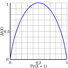
Figure 1:Entropy of a binary source
As an illustration of the property no.2 from above, we can see that the maximum entropy value of a DMS with two messages is reached when the two messages have the same probability, :
and its value is:
2.5Study case: games of guessing numbers
Let’s analyze the following guessing games with the tools introduced until now.
2.6Efficiency, redundancy, flow
Using the , we define several other useful characteristics of a DMS.
The efficiency of a DMS indicates how close is the entropy to its maximum possible value:
The redundancy of a source is the remaining gap. We can define an absolute redundancy and a relative redundancy.
Absolute redundancy of a DMS:
Relative redundancy of a DMS:
Suppose that each message takes some time to be transmitted via some communication channel. The information flow of a DMS is the average information transmitted per unit of time:
where is the average duration of transmitting a message:
The information flow is measured in bps (bits per second), and is important for data communication.
2.7The Kullback-Leibler distance
Suppose we have the following two DMS:
The probability values of and are close, so the two sources are similar. But exactly how similar? Can we quantify the “closeness” of the two sources?
In many application we need a way to quantify how similar or how different are two probability distributions. The Kullback-Leibler distance (also known as “Kullback-Leibler divergence”, or “cross-entropy”, or “relative entropy”) is a way to quantify numerically how much different is one distribution from another one.
The Kullback–Leibler (KL) distance of two distributions P and Q is:
The two distributions must have the same number of messages.
The KL distance provides a meaningful way to to measure the distance (difference) between two distributions. In many ways it provides the same intuitions as a geometrical distance:
is always , and is equal to 0 only when P and Q are the same
The higher is, the more different the two distributions are
However, one important property is not satisfied, and for this reason the KL distance is not proper distance function as defined e.g. in mathematical algebra. The KL distance is not commutative: :
Despite this, it is widely used in applications.
2.8Extended DMS
The n-th order extension of a DMS , represented as , is a DMS which has as messages all the combinations of messages of :
If has messages, has messages,
Since is DMS, consecutive messages are independent of each other, and therefore their probabilities are multiplied:
An example is provided below:
Extended DMS are useful because they provide a way to group messages inside a sequence of messages.
Suppose we have a long sequence of binary messages:
What kind of source generated this sequence?
We can view it as a sequence of 16 messages generated from a source with two messages, and
We can group two bits, and view it as a sequence of 8 messages generated from a source with messages 00, 01, 10, 11
We can group 8 bits into bytes, and view it is a sequence of 2 messages from a DMS which generates 256 bytes
... and so on
There must be a connection between the DMS, no matter how we group the bits, since we’re talking about the same binary sequence. The connections is that they are all just n-th order extensions of the initial binary DMS.
2.9Entropy of an extended DMS
We now prove an important theorem about extended DMS.
This theorem has a nice interpretation: when having a long sequence in of messages, we may group together blocks of messages as we like, this does not change total information of a sequence. This makes sense because we’re talking about the same sequence, even if we group bits into half-bytes, bytes, 32-bit words etc.
For example, imagine when we have a sequence of 1000 bits:
We can think of this sequence as being 1000 bits from a binary source which generates 0’s and 1’s. The total information in the sequence is .
However, if we group 8 bits into 1 byte, we can think of the same sequence as being 125 bytes from a source which produces bytes. This source is simply the extension of the original source , since its messages are just groupings of 8 messages from the original source. It’s entropy is therefore . Hence the total information in the sequence is the same: .
The theorem shows that both interpretations are correct. Grouping 8 messages of a source results in compound messages which are 8 times fewer, but carry 8 times more average information, so the total information is the same.
2.10DMS as models for language generation
We use information sources as mathematical models for real-life data generation and analysis. A straightforward example in in text analysis, since text is basically a sequence of graphical symbols (letters and punctuation signs), similar to a sequence of messages from an information source.
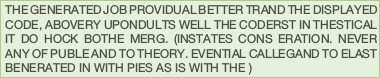
Is a DMS a good model for text? Let’s take the following example, for the English language. The probability distribution of letters in English (26 letters, ignoring capitalization) is given below [1]:
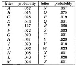
Figure 1:Probability distribution of letters in English
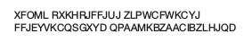
Let’s image a DMS which has the 26 letters as messages, with these probabilities. Generating a sequence of letters from this DMS produces the following:

Figure 1:Text generated from a DMS with English letter probabilities
This doesn’t look like English. What’s wrong?
A DMS is memoryless, which means that every message is generated irrespective
of the previous ones. This is not a good model for written text.
In a real language, the frequency of letter depends a lot on the previous letters.
Foe example, a is a common letter in English (probability ),
but if the previous letter is also a, the probability is close to zero
because the group aa is extremely rare. Similarly, h has
a much higher probability if the previous letter is t
then if the previous letter is x.
The DMS is not capturing the dependencies between letters, because the memoryless property makes it very restrictive. We need to consider sources with memory.
3Sources with memory
The last messages define the state of the source, which is denoted as . We say that the source “is in the state ”. Sources with memory are also known as Markov sources.
A source with messages and memory has a number of states equal to .
A source with memory generates messages randomly, but the message probabilities are different depending in which state the source is. We use the notation:
to refer to probability of message being generated when the source is in state . This is called the conditional probability of message given state .
3.1Transition matrix
When a new message is provided, the source transitions to a new state:
Therefore we can view the conditional probabilities of messages as transition probabilities from some state to another state . We can write:
which means that generating some message while in state is the same as transitioning into state from state .
The transition probabilities are organized in a transition matrix of size , where is the total number of states.
The element from , located on row and column , is the transition probability from state to state :
Note that the sum of the probabilities on each row is 1, because the source must move to some state after generating a message.
3.2Graphical representation
The transition matrix which defines a source with memory can be represented graphically, as a directed graph where the vertices are the states, and the edges are the transitions. Every edge (transition) has a certain probability,
The graphical representation of the previous example source is:
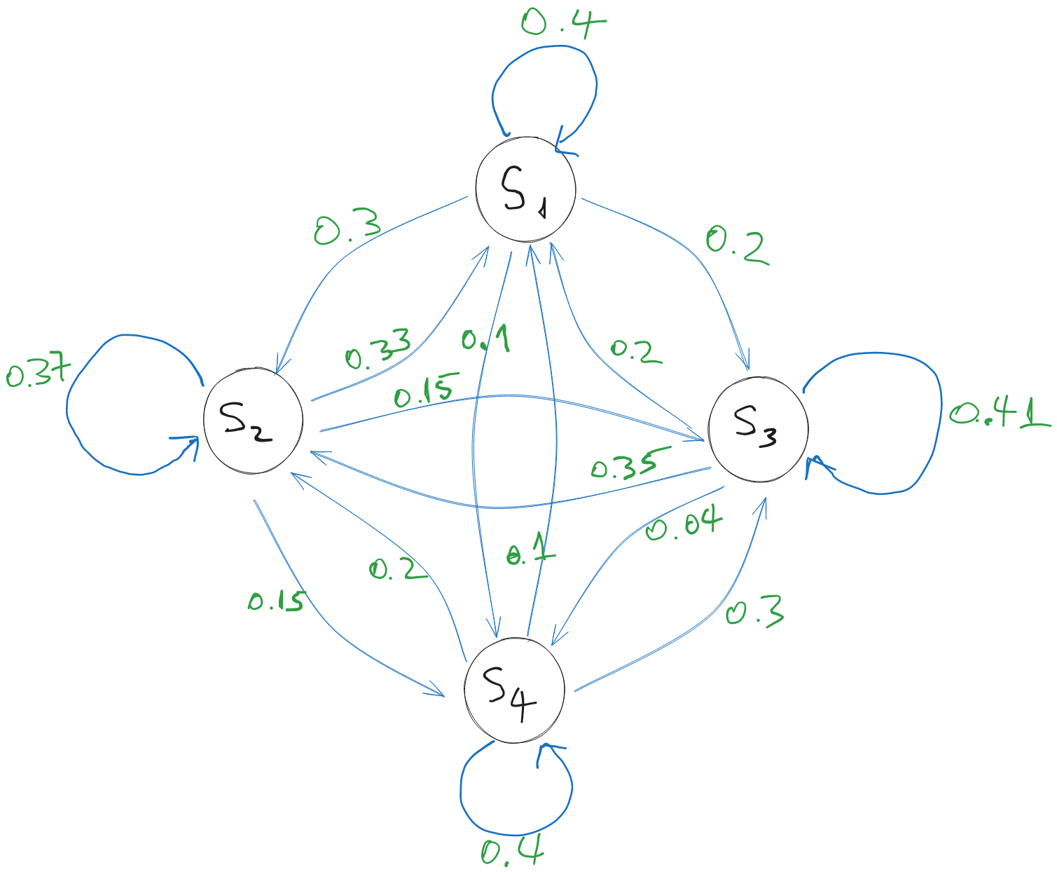
Figure 1:A source with memory and messages
For example, generating message while in state means we move from state to state (defined as last message ), so we have an arrow from to with probability 0.15.
Note that the sum of the probabilities of the transitions exiting from a state is 1, since the source must move to some state after generating a message. It is possible that the source stays in the same state, which is represented as a self-loop.
3.3Entropy of sources with memory
How to compute the entropy of a source with memory?
In each state there is different distribution, so each state can be viewed as a kind of DMS. We can compute an entropy for every state , using the same formula as for DMS:
However, is the entropy of a single state. While operating, the source moves from state to state, and it can spend more time in a state than in another one.
The global entropy of a source with memory is the average entropy of the states:
The probabilities are known as the stationary probabilities, and they represent the probability that the source is in state at a given moment. Considering that the source operates for a very long time and generates a very long sequence of messages, you can think of as the fraction of time when the source was in state .
Stationary probabilities
How to find out the stationary probabilities ? To find this, we first need to answer the following question:
If we know the state at time , what will be the state at time ?
Let denote the probability that the source is in state at time . The source generates a message. In what state will the source end up at time ?
The probabilities of the states at time , , are found by multiplying with
After one additional message, at time ? Multiply once more with :
For every new moment of time, we do one more multiplication with . In general, if we start from time 0, after messages, the probabilities that the source ends up in a certain state are:
However, in general we don’t know the initial state or the initial probabilities.
Ergodicity
To work around the problem of the unknown initial state, we make use a property called “ergodicity”.
If an ergodic source runs for a very long time , it will go through all transitions and all states many times, and, eventually, the fraction of time it finds itself in a certain state stabilizes. This happens irrespective of what was the starting state. Intuitively, the initial state is not important anymore if the source will anyway travel through all states and transitions many times, as .
We formalize this as the following property of an ergodic source with memory:
Finding the stationary probabilities
The ergodicity property helps us find the values of the stationary probabilities. When is very large, after messages and after messages the probabilities are the same, and therefore the following equation holds:
Note that we dropped the time exponent indicator or , since the values have converged to fixed values and the times doesn’t matter anymore.
This is an equation system in matrix form, with unknowns and equations.
However, the system is rank-deficient, i.e. one row is actually a linear combination of the others. Because of this, one row of the system should be removed, and replaced with a new equation which reflects the fact that the sum of probabilities is 1:
With this new equation, we obtain a complete system, which has a unique set of solutions by solving the system.
3.4Example: Modelling English
This example is taken from “Elements of Information Theory” by Cover & Thomas.
Let us consider a sequence of information sources modelling English language, going progressively from the most rudimentary model (memoryless), to the most advanced (source with memory of large order).
Let’s look at a sample sequence of letters generated from these sources.
Text generated by memoryless source, where all letters have equal probabilities:
A memoryless source, but the probabilities of each letter as the ones in English:
A source with memory of order , i.e. frequency of letter pairs are as in English:

A source with memory , i.e. the frequency of letter triplets as in English:

A source with memory , frequency of 4-plets as in English:
The generated text, while still random, gradually looks more and more like actual English as the memory order increases.
Sources with more memory are able to capture better the statistical dependencies between the letters, and because of this the generated text looks more and more like English.
3.5Working with information sources
When using information sources to model a real-life process, you will encounter some typical use-cases.
How to train an information source (e.g. find the probabilities)
Generate sequences from a source
Compute the probability of an existing sequence
Training an information source model
By training a model we mean finding the correct value of the parameters. In our case, the parameters are the probabilities of messages.
For simplicity, we consider the case of text analysis in a certain language (e.g. English).
First, we need a large sample of text, representative for the language.
How to find the probabilities of a DMS?
Go through your sample text, count the occurrences of every distinct character, then divide the counters to the total number of characters. You obtain the probabilities of each individual characters.
How to find the probabilities of a source with memory of order ?
A direct approach to find the transition matrix is as follows:
First, define each possible state . Let’s assume there are states.
Go though the sample text, count every occurrence of a group of distinct characters. Place the counters in an matrix , where each row corresponds to the old state (first characters of the group), and columns are the new state (last characters of the group).
Normalize each row: divide each row to the sum of the row. This ensures that the resulting row sums up to 1, i.e. it forms a probability distribution.
One drawback is the huge memory requirements required to count all the possible combinations. The memory requirement increases at least exponentially with the memory order . For example, if there are 26 letters, a source with memory of order has states, while a source with has states. Considering capital letters and punctuation signs, the numbers are much larger. This makes it very cumbersome to work with sources of large memory, at least with such a brute-force approach.
Generating messages from a source
Supposing we have a source, we generate sequences by generating messages one after another.
For a DMS, we generate each message independently of all the previous ones.
For a source with memory , described by a transition matrix , we generate a message according to the transition probabilities from the row of corresponding to the current state. Then we update the current state and repeat the process.
For a source with memory, we must also specify how to generate the first messages, i.e. before we have the first previous messages which define a full state.
Compute the probability of an existing sequence
Suppose we have a sequence Seq of messages, e.g.
“wirtschaftwissenschaftler”
If we have an information source, how do we compute the probability that the sequence Seq was generated from the source?
For a DMS, simply multiply the probabilities of every letter in the sequence
For a DMS with memory , look at every group of letters and multiply the corresponding probabilities from the transition matrix
Multiplying many probabilities quickly results in a very small number, which makes it problematic on a digital device due to numerical errors.
To avoid this, instead of probabilities we can work with the log-probabilities, i.e. , which allows for much more manageable values. Instead of multiplying probabilities, we sum the log-probabilities.
3.6Sample applications
Predict text
Suppose we receive a text with random missing letters
We need to fill the blanks with the appropriate letters
How?
build a model: source with memory of some order
fill the missing letter with the most likely letter given by the model
Guess language of a sentence
We have piece of text. What language is it written in?
We model each language with a source with memory, each trained on a sufficiently large piece of text representative of the language
We compute the log-probability of the text with every language source model. Pick the one with the highest value.
Image is taken from the book “Elements of Information Theory" by Cover, Thomas”