a). compute the marginal probabilities and the marginal entropies H(X) and H(Y)
The marginal probabilities are computed by summing the joint probabilities over the rows and columns.
The rows correspond to the inputs xi, and the columns correspond to the outputs yj.
The marginal probabilities p(xi) are found by summing the rows:
b). Find the channel matrix P(Y∣X) and draw the graph of the channel
The channel matrix P(Y∣X) is computed by dividing each row of the joint probability matrix
by the corresponding p(xi), i.e. by the sum of that row.
This is known as “normalization” of the rows.
The resulting matrix contains the conditional probabilities P(yj∣xi).
Dividing the first row by p(x1)=21 and the second row by p(x2)=21, we get:
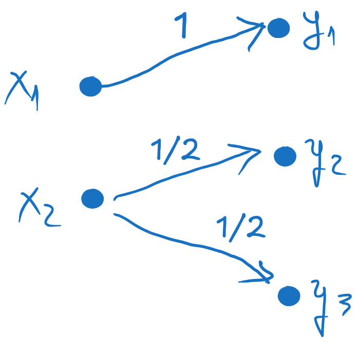
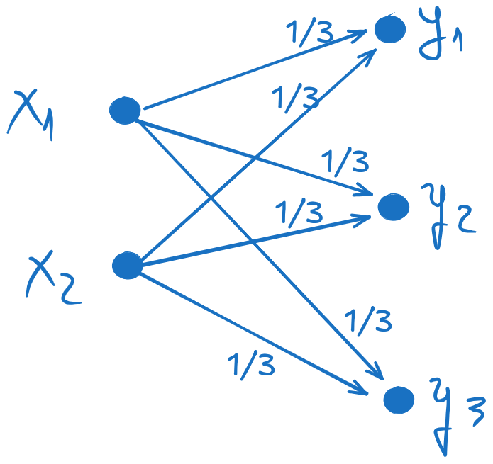
The graph of the channel is a graphical representation of the channel matrix,
where the inputs xi are on the left, the outputs yj are on the right,
and the non-zero probabilities are shown as arrows from inputs to outputs.
c). compute the mutual information I(X,Y), and draw the geometrical representation
We start from the general relation between the six entropies,
discussed in the lecture:
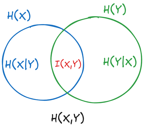
Figure 2:General relation between the six entropies
where:
H(X) is the area of the first circle
H(Y) is the area of the second circle
H(X,Y) is the area of the reunion of the two circles
H(X∣Y) is the part of the first circle outside of the second circle
H(Y∣X) is the part of the second circle outside of the first circle
I(X,Y) is the intersection of the two circles
Knowing three of the six entropies, we can compute the other three using
relations deduced from the figure.
In this case, we already know H(X)=1 and H(Y)=1.5 from a).
Another easy one is H(X,Y), which is the entropy of all the values in the joint probability matrix:
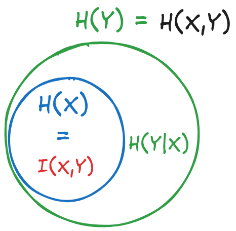
For the geometrical representation,
we observe that H(X,Y) is equal to H(Y),
which means that the first circle is completely contained in the second circle.
Figure 3:Geometrical representation of the entropies for Exercise 1
We first need to compute the joint probability matrix P(xi∩yj).
We do this by multiplying the rows of the channel matrix P(Y∣X) by the probabilities of the inputs p(xi), each row by the corresponding p(xi).
This is the opposite of the normalization we did in Exercise 1.
We multiply the first row by p(x1)=43 and the second row by p(x2)=41:
c). Compute the uncertainty remaining over the input X when output symbol y2 is received
“The uncertainty remaining over the input X when output symbol y2 is received”
is the conditional entropy H(X∣y2).
This is the entropy of the second column (y2) from the matrix P(X∣Y).
To compute the matrix P(X∣Y), we need to normalize the columns joint probability matrix P(xi∩yj) (i.e. divide each column by its sum, the corresponding marginal probability p(yj)).
Normalizing the columns of the joint probability matrix, we get:
We use the fact that the channel is symmetric, i.e. it is uniform with respect to the input
and also uniform with respect to the output (see the lecture for more on this).
Since the channel is uniform with respect to the input, H(Y∣X) does
not depend on the input probabilities p(xi), and is constant (see lectures).
As such, it goes out of the maximization above, and we can write:
The entropy H(Y) is maximum when the probabilities p(yj) are equal.
Since the channel is also uniform with respect to the output,
the consequence is that “If the input symbols are equiprobable, the output symbols are also
equiprobable” (see the lecture).
Therefore, the maximum value of H(Y) is achieved when p(x1)=p(x2)=21,
which implies that p(y1)=p(y2)=21.
Therefore, the maximum value of H(Y) is:
Since the inputs and outputs have equal probabilities, it means that
p(x1)=p(x2)=21 and p(y1)=p(y2)=p(y3)=31.
The joint probability matrix is then:
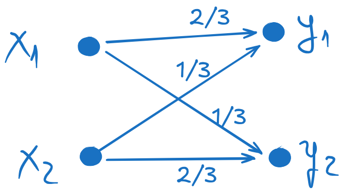
b). Draw the graph of the channel (together with the probabilities)
We obtain the channel matrix P(Y∣X) by dividing each row of the joint probability matrix
to its corresponding marginal probability p(xi).
This results in:
c). Compute the marginal entropies and the joint entropy, and verify that H(X,Y)=H(X)+H(Y) and that I(X,Y)=0
We know the probabilities p(xi) and p(yj), so we can compute the marginal entropies.
The joint entropy H(X,Y) is computed from all the six values in the joint probability matrix.
This is to be expected, since the inputs and outputs are independent,
and this means that there is no relation between the inputs and outputs of the channel.
Therefore the communication is useless, and no information is transmitted at all.
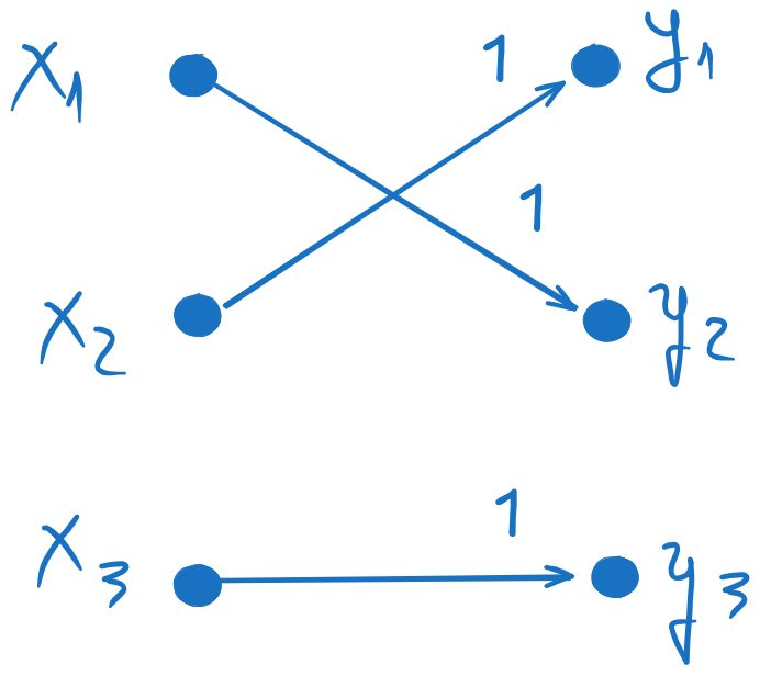
3 inputs and 3 outputs means a channel matrix P(Y∣X) with 3 rows and 3 columns.
H(Y∣X)=0 means zero uncertainty about the output when the input is known.
This means that there is a single arrow from each input xi to a single output yj.
The probability must then be 1.
H(Y∣x1) is the entropy computed from the first row of the channel matrix P(Y∣X).
It must be non-zero, which means that there should be at least two non-zero probabilities.
H(Y∣x2)0 is the entropy computed from the second row of the channel matrix P(Y∣X),
and since it is zero, there must be a single value of 1 and all the others must be 0.
Therefore, a possible channel matrix, with two inputs and two outputs, is: